


Woodwinds
We now consider models of woodwind instruments, focusing on the single-reed case. In §9.5.4, tonehole modeling is described in some detail.
Single-Reed Instruments
A simplified model for a single-reed woodwind instrument is shown in Fig. 9.38 [431].
![\includegraphics[width=\twidth]{eps/fSingleReedAI}](http://www.dsprelated.com/josimages_new/pasp/img2307.png)
If the bore is cylindrical, as in the clarinet, it can be modeled quite simply using a bidirectional delay line. If the bore is conical, such as in a saxophone, it can still be modeled as a bidirectional delay line, but interfacing to it is slightly more complex, especially at the mouthpiece [37,7,160,436,506,507,502,526,406,528], Because the main control variable for the instrument is air pressure in the mouth at the reed, it is convenient to choose pressure wave variables.
To first order, the bell passes high frequencies and reflects low
frequencies, where ``high'' and ``low'' frequencies are divided by the
wavelength which equals the bell's diameter. Thus, the bell can be regarded
as a simple ``cross-over'' network, as is used to split signal energy
between a woofer and tweeter in a loudspeaker cabinet. For a clarinet
bore, the nominal ``cross-over frequency'' is around ![]() Hz
[38]. The flare of the bell lowers the cross-over frequency by
decreasing the bore characteristic impedance toward the end in an
approximately non-reflecting manner [51]. Bell flare can
therefore be
considered analogous to a transmission-line transformer.
Hz
[38]. The flare of the bell lowers the cross-over frequency by
decreasing the bore characteristic impedance toward the end in an
approximately non-reflecting manner [51]. Bell flare can
therefore be
considered analogous to a transmission-line transformer.
Since the length of the clarinet bore is only a quarter wavelength at the fundamental frequency, (in the lowest, or ``chalumeau'' register), and since the bell diameter is much smaller than the bore length, most of the sound energy traveling into the bell reflects back into the bore. The low-frequency energy that makes it out of the bore radiates in a fairly omnidirectional pattern. Very high-frequency traveling waves do not ``see'' the enclosing bell and pass right through it, radiating in a more directional beam. The directionality of the beam is proportional to how many wavelengths fit along the bell diameter; in fact, many wavelengths away from the bell, the radiation pattern is proportional to the two-dimensional spatial Fourier transform of the exit aperture (a disk at the end of the bell) [308].
The theory of the single reed is described, e.g., in [102,249,308]. In the digital waveguide clarinet model described below [431], the reed is modeled as a signal- and embouchure-dependent nonlinear reflection coefficient terminating the bore. Such a model is possible because the reed mass is neglected. The player's embouchure controls damping of the reed, reed aperture width, and other parameters, and these can be implemented as parameters on the contents of the lookup table or nonlinear function.
Digital Waveguide Single-Reed Implementation
A diagram of the basic clarinet model is shown in
Fig.9.39. The delay-lines carry left-going and
right-going pressure samples ![]() and
and ![]() (respectively) which
sample the traveling pressure-wave components within the bore.
(respectively) which
sample the traveling pressure-wave components within the bore.
![\includegraphics[width=\twidth]{eps/fSingleReedWGM}](http://www.dsprelated.com/josimages_new/pasp/img2311.png)
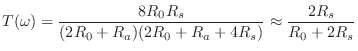
The reflection filter at the right implements the bell or tone-hole
losses as well as the round-trip attenuation losses from traveling
back and forth in the bore. The bell output filter is highpass, and
power complementary with respect to the bell reflection filter
[500]. Power complementarity follows from the
assumption that the bell itself does not vibrate or otherwise absorb
sound. The bell is also amplitude complementary. As a result,
given a reflection filter ![]() designed to match measured mode
decay-rates in the bore, the transmission filter can be written down
simply as
designed to match measured mode
decay-rates in the bore, the transmission filter can be written down
simply as
![]() for velocity waves, or
for velocity waves, or
![]() for pressure waves. It is easy to show that such
amplitude-complementary filters are also power complementary by
summing the transmitted and reflected power waves:
for pressure waves. It is easy to show that such
amplitude-complementary filters are also power complementary by
summing the transmitted and reflected power waves:
![\begin{eqnarray*}
P_t U_t + P_r U_r &=& (1+H_r)P \cdot (1-H_r)U + H_r P \cdot (-H_r)(-U)\\
&=& [1-H_r^2 + H_r^2]PU \;=\; PU,
\end{eqnarray*}](http://www.dsprelated.com/josimages_new/pasp/img2315.png)
where ![]() denotes the z transform transform of the incident pressure wave,
and
denotes the z transform transform of the incident pressure wave,
and ![]() denotes the z transform of the incident volume-velocity. (All
z transform have omitted arguments
denotes the z transform of the incident volume-velocity. (All
z transform have omitted arguments
![]() , where
, where
![]() denotes the sampling interval in seconds.)
denotes the sampling interval in seconds.)
At the far left is the reed mouthpiece controlled by mouth
pressure ![]() . Another control is embouchure, changed in
general by modifying the reflection-coefficient function
. Another control is embouchure, changed in
general by modifying the reflection-coefficient function
![]() , where
, where
![]() . A simple choice of embouchure control is an
offset in the reed-table address. Since the main feature of the reed table
is the pressure-drop where the reed begins to open, a simple embouchure
offset can implement the effect of biting harder or softer on the reed, or
changing the reed stiffness.
. A simple choice of embouchure control is an
offset in the reed-table address. Since the main feature of the reed table
is the pressure-drop where the reed begins to open, a simple embouchure
offset can implement the effect of biting harder or softer on the reed, or
changing the reed stiffness.
A View of Single-Reed Oscillation
To start the oscillation, the player applies a pressure at the mouthpiece which ``biases'' the reed in a ``negative-resistance'' region. (The pressure drop across the reed tends to close the air gap at the tip of the reed so that an increase in pressure will result in a net decrease in volume velocity--this is negative resistance.) The high-pressure front travels down the bore at the speed of sound until it encounters an open air hole or the bell. To a first approximation, the high-pressure wave reflects with a sign inversion and travels back up the bore. (In reality a lowpass filtering accompanies the reflection, and the complementary highpass filter shapes the spectrum that emanates away from the bore.)
As the negated pressure wave travels back up the bore, it cancels the elevated pressure that was established by the passage of the first wave. When the negated pressure front gets back to the mouthpiece, it is reflected again, this time with no sign inversion (because the mouthpiece looks like a closed end to a first approximation). Therefore, as the wave travels back down to the bore, a negative pressure zone is left behind. Reflecting from the open end again with a sign inversion brings a return-to-zero wave traveling back to the mouthpiece. Finally the positive traveling wave reaches the mouthpiece and starts the second ``period'' of oscillation, after four trips along the bore.
So far, we have produced oscillation without making any use of the negative-resistance of the reed aperture. This is merely the start-up transient. Since in reality there are places of pressure loss in the bore, some mechanism is needed to feed energy back into the bore and prevent the oscillation just described from decaying exponentially to zero. This is the function of the reed: When a traveling pressure-drop reflects from the mouthpiece, making pressure at the mouthpiece switch from high to low, the reed changes from open to closed (to first order). The closing of the reed increases the reflection coefficient ``seen'' by the impinging traveling wave, and so as the pressure falls, it is amplified by an increasing gain (whose maximum is unity when the reed shuts completely). This process sharpens the falling edge of the pressure drop. But this is not all. The closing of the reed also cuts back on the steady incoming flow from the mouth. This causes the pressure to drop even more, potentially providing effective amplification by more than unity.
An analogous story can be followed through for a rising pressure appearing at the mouthpiece. However, in the rising pressure case, the reflection coefficient falls as the pressure rises, resulting in a progressive attenuation of the reflected wave; however, the increased pressure let in from the mouth amplifies the reflecting wave. It turns out that the reflection of a positive wave is boosted when the incoming wave is below a certain level and it is attenuated above that level. When the oscillation reaches a very high amplitude, it is limited on the negative side by the shutting of the reed, which sets a maximum reflective amplification for the negative excursions, and it is limited on the positive side by the attenuation described above. Unlike classical negative-resistance oscillators, in which the negative-resistance device is terminated by a simple resistance instead of a lossy transmission line, a dynamic equilibrium is established between the amplification of the negative excursion and the dissipation of the positive excursion.
In the first-order case, where the reflection-coefficient varies linearly with pressure drop, it is easy to obtain an exact quantitative description of the entire process. In this case it can be shown, for example, that amplification occurs only on the positive half of the cycle, and the amplitude of oscillation is typically close to half the incoming mouth pressure (when losses in the bore are small). The threshold blowing pressure (which is relatively high in this simplified case) can also be computed in closed form.
Single-Reed Theory
![\includegraphics[scale=0.9]{eps/fReedSchematic}](http://www.dsprelated.com/josimages_new/pasp/img2321.png)
A simplified diagram of the clarinet mouthpiece is shown in
Fig. 9.40. The pressure in the mouth is assumed
to be a constant value ![]() , and the bore pressure
, and the bore pressure ![]() is defined
located at the mouthpiece. Any pressure drop
is defined
located at the mouthpiece. Any pressure drop
![]() across
the mouthpiece causes a flow
across
the mouthpiece causes a flow ![]() into the mouthpiece through the
reed-aperture impedance
into the mouthpiece through the
reed-aperture impedance
![]() which changes as a function of
which changes as a function of
![]() since the reed position is affected by
since the reed position is affected by
![]() . To a first
approximation, the clarinet reed can be regarded as a spring flap
regulated Bernoulli flow (§B.7.5), [249]).
This model has been verified well experimentally until the reed is
about to close, at which point viscosity effects begin to appear
[102]. It has also been verified that the mass
of the reed can be neglected to first order,10.18 so that
. To a first
approximation, the clarinet reed can be regarded as a spring flap
regulated Bernoulli flow (§B.7.5), [249]).
This model has been verified well experimentally until the reed is
about to close, at which point viscosity effects begin to appear
[102]. It has also been verified that the mass
of the reed can be neglected to first order,10.18 so that
![]() is a
positive real number for all values of
is a
positive real number for all values of
![]() . Possibly the most
important neglected phenomenon in this model is sound generation due
to turbulence of the flow, especially near reed closure. Practical
synthesis models have always included a noise component of some sort
which is modulated by the reed [431], despite a lack of firm
basis in acoustic measurements to date.
. Possibly the most
important neglected phenomenon in this model is sound generation due
to turbulence of the flow, especially near reed closure. Practical
synthesis models have always included a noise component of some sort
which is modulated by the reed [431], despite a lack of firm
basis in acoustic measurements to date.
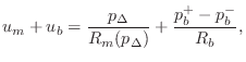
The fundamental equation governing the action of the reed is continuity of volume velocity, i.e.,
where
and
is the volume velocity corresponding to the incoming pressure wave
In operation, the mouth pressure ![]() and incoming traveling bore pressure
and incoming traveling bore pressure
![]() are given, and the reed computation must produce an outgoing bore
pressure
are given, and the reed computation must produce an outgoing bore
pressure ![]() which satisfies (9.35), i.e., such that
which satisfies (9.35), i.e., such that
Solving for
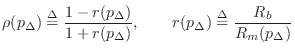
It is helpful to normalize (9.38) as follows: Define
![]() , and note that
, and note that
![]() , where
, where
![]() . Then (9.38) can be multiplied through by
. Then (9.38) can be multiplied through by ![]() and
written as
and
written as
![]() , or
, or
The solution is obtained by plotting
| (10.40) |
An example of the qualitative appearance of ![]() overlaying
overlaying
![]() is shown in Fig. 9.41.
is shown in Fig. 9.41.
![\includegraphics[width=\twidth]{eps/fReedRelations}](http://www.dsprelated.com/josimages_new/pasp/img2346.png)
Scattering-Theoretic Formulation
Equation (9.38) can be solved for ![]() to obtain
to obtain

where
 |
(10.44) |
We interpret
Since the mouthpiece of a clarinet is nearly closed,
![]() which
implies
which
implies
![]() and
and
![]() . In the limit as
. In the limit as ![]() goes to
infinity relative to
goes to
infinity relative to ![]() , (9.42) reduces to the simple form of a
rigidly capped acoustic tube, i.e.,
, (9.42) reduces to the simple form of a
rigidly capped acoustic tube, i.e.,
![]() .
If it were possible to open the reed wide enough to achieve
matched impedance,
.
If it were possible to open the reed wide enough to achieve
matched impedance, ![]() , then we would have
, then we would have ![]() and
and ![]() , in
which case
, in
which case
![]() , with no reflection of
, with no reflection of ![]() , as expected. If
the mouthpiece is removed altogether to give
, as expected. If
the mouthpiece is removed altogether to give ![]() (regarding it now as a
tube section of infinite radius), then
(regarding it now as a
tube section of infinite radius), then ![]() ,
, ![]() , and
, and
![]() .
.
Computational Methods
Since finding the intersection of ![]() and
and
![]() requires an expensive
iterative algorithm with variable convergence times, it is not well suited
for real-time operation. In this section, fast algorithms based on
precomputed nonlinearities are described.
requires an expensive
iterative algorithm with variable convergence times, it is not well suited
for real-time operation. In this section, fast algorithms based on
precomputed nonlinearities are described.
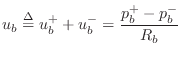
Let ![]() denote half-pressure
denote half-pressure ![]() , i.e.,
, i.e.,
![]() and
and
![]() . Then (9.43) becomes
. Then (9.43) becomes
Subtracting this equation from
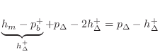
The last expression above can be used to precompute
| (10.47) |
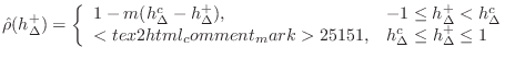
(9.45) becomes
This is the form chosen for implementation in Fig. 9.39 [431]. The control variable is mouth half-pressure
Because the table contains a coefficient rather than a signal value, it
can be more heavily quantized both in address space and word length than
a direct lookup of a signal value such as
![]() or the like. A
direct signal lookup, though requiring much higher resolution, would
eliminate the multiplication associated with the scattering coefficient.
For example, if
or the like. A
direct signal lookup, though requiring much higher resolution, would
eliminate the multiplication associated with the scattering coefficient.
For example, if ![]() and
and ![]() are 16-bit signal samples,
the table would contain on the order of 64K 16-bit
are 16-bit signal samples,
the table would contain on the order of 64K 16-bit
![]() samples.
Clearly, some compression of this table would be desirable. Since
samples.
Clearly, some compression of this table would be desirable. Since
![]() is smoothly varying, significant compression is in fact
possible. However, because the table is directly in the signal path,
comparatively little compression can be done while maintaining full
audio quality (such as 16-bit accuracy).
is smoothly varying, significant compression is in fact
possible. However, because the table is directly in the signal path,
comparatively little compression can be done while maintaining full
audio quality (such as 16-bit accuracy).
![\includegraphics[width=4in]{eps/fReedTable}](http://www.dsprelated.com/josimages_new/pasp/img2382.png)
In the field of computer music, it is customary to use simple piecewise linear functions for functions other than signals at the audio sampling rate, e.g., for amplitude envelopes, FM-index functions, and so on [382,380]. Along these lines, good initial results were obtained [431] using the simplified qualitatively chosen reed table
depicted in Fig. 9.42 for
Another variation is to replace the table-lookup contents by a piecewise polynomial approximation. While less general, good results have been obtained in practice [89,91,92]. For example, one of the SynthBuilder [353] clarinet patches employs this technique using a cubic polynomial.
An intermediate approach between table lookups and polynomial approximations is to use interpolated table lookups. Typically, linear interpolation is used, but higher order polynomial interpolation can also be considered (see Chapter 4).
Clarinet Synthesis Implementation Details
To finish off the clarinet example, the remaining details of the SynthBuilder clarinet patch Clarinet2.sb are described.
The input mouth pressure is summed with a small amount of white noise,
corresponding to turbulence. For example, 0.1% is generally used as a
minimum, and larger amounts are appropriate during the attack of a note.
Ideally, the turbulence level should be computed automatically as a
function of pressure drop
![]() and reed opening geometry
[141,530]. It should also be lowpass filtered
as predicted by theory.
and reed opening geometry
[141,530]. It should also be lowpass filtered
as predicted by theory.
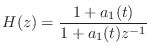
Referring to Fig. 9.39, the reflection filter is a simple one-pole with transfer function
 |
(10.50) |
where
Legato note transitions are managed using two delay line taps and cross-fading from one to the other during a transition [208,441,405]. In general, legato problems arise when the bore length is changed suddenly while sounding, corresponding to a new fingering. The reason is that really the model itself should be changed during a fingering change from that of a statically terminated bore to that of a bore with a new scattering junction appearing where each ``finger'' is lifting, and with disappearing scattering junctions where tone holes are being covered. In addition, if a hole is covered abruptly (especially when there are large mechanical caps, as in the saxophone), there will also be new signal energy injected in both directions on the bore in superposition with the signal scattering. As a result of this ideal picture, is difficult to get high quality legato performance using only a single delay line.
A reduced-cost, approximate solution for obtaining good sounding note transitions in a single delay-line model was proposed in [208]. In this technique, the bore delay line is ``branched'' during the transition, i.e., a second feedback loop is formed at the new loop delay, thus forming two delay lines sharing the same memory, one corresponding to the old pitch and the other corresponding to the new pitch. A cross-fade from the old-pitch delay to the new-pitch delay sounds good if the cross-fade time and duration are carefully chosen. Another way to look at this algorithm is in terms of ``read pointers'' and ``write pointers.'' A normal delay line consists of a single write pointer followed by a single read pointer, delayed by one period. During a legato transition, we simply cross-fade from a read-pointer at the old-pitch delay to a read-pointer at the new-pitch delay. In this type of implementation, the write-pointer always traverses the full delay memory corresponding to the minimum supported pitch in order that read-pointers may be instantiated at any pitch-period delay at any time. Conceptually, this simplified model of note transitions can be derived from the more rigorous model by replacing the tone-hole scattering junction by a single reflection coefficient.
STK software implementing a model as in Fig.9.39 can be found in the file Clarinet.cpp.
Tonehole Modeling
Toneholes in woodwind instruments are essentially cylindrical holes in
the bore. One modeling approach would be to treat the tonehole as a
small waveguide which connects to the main bore via one port on a
three-port junction. However, since the tonehole length is small
compared with the distance sound travels in one sampling instant (
![]() in, e.g.), it is more straightforward to treat the
tonehole as a lumped load along the bore, and most modeling efforts
have taken this approach.
in, e.g.), it is more straightforward to treat the
tonehole as a lumped load along the bore, and most modeling efforts
have taken this approach.
The musical acoustics literature contains experimentally verified models of tone-hole acoustics, such as by Keefe [238]. Keefe's tonehole model is formulated as a ``transmission matrix'' description, which we may convert to a traveling-wave formulation by a simple linear transformation (described in §9.5.4 below) [465]. For typical fingerings, the first few open tone holes jointly provide a bore termination [38]. Either the individual tone holes can be modeled as (interpolated) scattering junctions, or the whole ensemble of terminating tone holes can be modeled in aggregate using a single reflection and transmission filter, like the bell model. Since the tone hole diameters are small compared with most audio frequency wavelengths, the reflection and transmission coefficients can be implemented to a reasonable approximation as constants, as opposed to cross-over filters as in the bell. Taking into account the inertance of the air mass in the tone hole, the tone hole can be modeled as a two-port loaded junction having load impedance equal to the air-mass inertance [143,509]. At a higher level of accuracy, adapting transmission-matrix parameters from the existing musical acoustics literature leads to first-order reflection and transmission filters [238,406,403,404,465]. The individual tone-hole models can be simple lossy two-port junctions, modeling only the internal bore loss characteristics, or three-port junctions, modeling also the transmission characteristics to the outside air. Another approach to modeling toneholes is the ``wave digital'' model [527] (see §F.1 for a tutorial introduction to this approach). The subject of tone-hole modeling is elaborated further in [406,502]. For simplest practical implementation, the bell model can be used unchanged for all tunings, as if the bore were being cut to a new length for each note and the same bell were attached. However, for best results in dynamic performance, the tonehole model should additionally include an explicit valve model for physically accurate behavior when slowly opening or closing the tonehole [405].
The Clarinet Tonehole as a Two-Port Junction
![\includegraphics[scale=0.9]{eps/fFingerHoleKeefe}](http://www.dsprelated.com/josimages_new/pasp/img2398.png)
The clarinet tonehole model developed by Keefe [240] is
parametrized in terms of series and shunt resistance and reactance, as
shown in Fig. 9.43. The transmission
matrix description of this two-port is given by the product of the
transmission matrices for the series impedance ![]() , shunt
impedance
, shunt
impedance ![]() , and series impedance
, and series impedance ![]() , respectively:
, respectively:
![$\displaystyle \left[\begin{array}{c} P_1 \\ [2pt] U_1 \end{array}\right]$](http://www.dsprelated.com/josimages_new/pasp/img2401.png)
![$\displaystyle \left[\begin{array}{cc} 1 & R_a/2 \\ [2pt] 0 & 1 \end{array}\righ...
...1 \end{array}\right]
\left[\begin{array}{c} P_2 \\ [2pt] U_2 \end{array}\right]$](http://www.dsprelated.com/josimages_new/pasp/img2402.png)
![$\displaystyle \left[\begin{array}{cc} 1+\frac{R_a}{2R_s} & R_a[1+\frac{R_a}{4R_...
...} \end{array}\right]
\left[\begin{array}{c} P_2 \\ [2pt] U_2 \end{array}\right]$](http://www.dsprelated.com/josimages_new/pasp/img2403.png)
where all quantities are written in the frequency domain, and the impedance parameters are given by
| (open-hole shunt impedance) |
|||
| (closed-hole shunt impedance) |
(10.51) | ||
| (open-hole series impedance) |
|||
| (closed-hole series impedance) |
where
 |
|||
 |
where
![$\displaystyle t_h = t_w + \frac{1}{8}\frac{b^2}{a}\left[1+0.172\left(\frac{b}{a}\right)^2\right]
$](http://www.dsprelated.com/josimages_new/pasp/img2426.png)
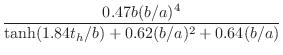
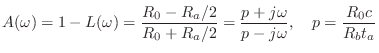
Note that the specific resistance of the open tonehole, ![]() , is the
only real impedance and therefore the only source of wave energy loss at
the tonehole. It is given by [240]
, is the
only real impedance and therefore the only source of wave energy loss at
the tonehole. It is given by [240]

![$\displaystyle \alpha = \frac{1}{2bc}\left[\,\sqrt{\frac{2\eta\omega}{\rho}}
+ (\gamma-1)\sqrt{\frac{2\kappa\omega}{\rho C_p}}\,\right]
$](http://www.dsprelated.com/josimages_new/pasp/img2433.png)
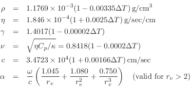
where
The open-hole effective length ![]() , assuming no pad above the hole,
is given in
[240] as
, assuming no pad above the hole,
is given in
[240] as
![$\displaystyle t_e = \frac{(1/k)\tan(kt) + b [1.40 - 0.58(b/a)^2]}{1 - 0.61 kb \tan(kt)}
$](http://www.dsprelated.com/josimages_new/pasp/img2445.png)
For implementation in a digital waveguide model, the lumped parameters above must be converted to scattering parameters. Such formulations of toneholes have appeared in the literature: Vesa Välimäki [509,502] developed tonehole models based on a ``three-port'' digital waveguide junction loaded by an inertance, as described in Fletcher and Rossing [143], and also extended his results to the case of interpolated digital waveguides. It should be noted in this context, however, that in the terminology of Appendix C, Välimäki's tonehole representation is a loaded 2-port junction rather than a three-port junction. (A load can be considered formally equivalent to a ``waveguide'' having wave impedance given by the load impedance.) Scavone and Smith [402] developed digital waveguide tonehole models based on the more rigorous ``symmetric T'' acoustic model of Keefe [240], using general purpose digital filter design techniques to obtain rational approximations to the ideal tonehole frequency response. A detailed treatment appears in Scavone's CCRMA Ph.D. thesis [406]. This section, adapted from [465], considers an exact translation of the Keefe tonehole model, obtaining two one-filter implementations: the ``shared reflectance'' and ``shared transmittance'' forms. These forms are shown to be stable without introducing an approximation which neglects the series inertance terms in the tonehole model.
By substituting
![]() in (9.53) to convert spatial
frequency to temporal frequency, and by substituting
in (9.53) to convert spatial
frequency to temporal frequency, and by substituting
| (10.52) | |||
 |
(10.53) |
for
        Clear["t*", "p*", "u*", "r*"]
        transmissionMatrix = {{t11, t12}, {t21, t22}};
        leftPort = {{p2p+p2m}, {(p2p-p2m)/r2}};
        rightPort = {{p1p+p1m}, {(p1p-p1m)/r1}};
        Format[t11, TeXForm] := "{T_{11}}"
        Format[p1p, TeXForm] := "{P_1^+}"
        ... (etc. for all variables) ...
        TeXForm[Simplify[Solve[leftPort ==
               transmissionMatrix . rightPort, {p1m, p2p}]]]
The above code produces the following formulas:
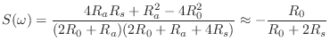
Substituting relevant values for Keefe's tonehole model, we obtain, in matrix notation,
![$\displaystyle \left[\begin{array}{c} P_1^{-} \\ [2pt] P_2^{+} \end{array}\right]$](http://www.dsprelated.com/josimages_new/pasp/img2459.png)
![$\displaystyle \left[\begin{array}{cc} S & T \\ [2pt] T & S \end{array}\right]
\left[\begin{array}{c} P_1^{+} \\ [2pt] P_2^{-} \end{array}\right]$](http://www.dsprelated.com/josimages_new/pasp/img2460.png)
![$\displaystyle \quad
\left[\begin{array}{cc} 4R_aR_s + R_a^2 - 4R_0^2 & 8R_0R_s ...
...rray}\right]
\left[\begin{array}{c} P_1^{+} \\ [2pt] P_2^{-} \end{array}\right]$](http://www.dsprelated.com/josimages_new/pasp/img2462.png)
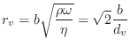
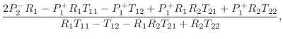
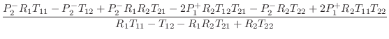
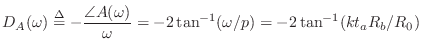
We thus obtain the scattering formulation depicted in Fig. 9.44, where
is the reflectance of the tonehole (the same from either direction), and
is the transmittance of the tonehole (also the same from either direction). The notation ``
![\includegraphics[scale=0.9]{eps/fFingerHoleScat}](http://www.dsprelated.com/josimages_new/pasp/img2465.png)
The approximate forms in (9.57) and (9.58) are obtained by neglecting
the negative series inertance ![]() which serves to adjust the effective
length of the bore, and which therefore can be implemented elsewhere in the
interpolated delay-line calculation as discussed further below. The open
and closed tonehole cases are obtained by substituting
which serves to adjust the effective
length of the bore, and which therefore can be implemented elsewhere in the
interpolated delay-line calculation as discussed further below. The open
and closed tonehole cases are obtained by substituting
![]() and
and
![]() , respectively, from (9.53).
, respectively, from (9.53).
In a manner analogous to converting the four-multiply Kelly-Lochbaum (KL)
scattering junction
[245]
into a one-multiply form (cf. (C.60) and
(C.62) on page ![]() ), we may pursue a ``one-filter'' form of the waveguide
tonehole model. However, the series inertance gives some initial trouble,
since
), we may pursue a ``one-filter'' form of the waveguide
tonehole model. However, the series inertance gives some initial trouble,
since
![$\displaystyle [1+S(\omega)] - T(\omega) = \frac{2R_a}{2R_0+ R_a} \isdef L(\omega)
$](http://www.dsprelated.com/josimages_new/pasp/img2469.png)
| (10.58) |
and, similarly,
| (10.59) |
The resulting tonehole implementation is shown in Fig. 9.45. We call this the ``shared reflectance'' form of the tonehole junction.
In the same way, an alternate form is obtained from the substitution
| (10.60) | |||
| (10.61) |
shown in Fig. 9.46.
![\includegraphics[scale=0.9]{eps/fFingerHoleOneMul}](http://www.dsprelated.com/josimages_new/pasp/img2485.png)
![\includegraphics[scale=0.9]{eps/fFingerHoleOneMulAlt}](http://www.dsprelated.com/josimages_new/pasp/img2486.png)
![\includegraphics[scale=0.9]{eps/fFingerHoleOneMulCommuted}](http://www.dsprelated.com/josimages_new/pasp/img2487.png) |
![\includegraphics[width=\twidth]{eps/fFingerHoleOneMulAltCommuted}](http://www.dsprelated.com/josimages_new/pasp/img2488.png)
Since
![]() , it can be neglected to first order, and
, it can be neglected to first order, and
![]() , reducing both of the above forms to an approximate
``one-filter'' tonehole implementation.
, reducing both of the above forms to an approximate
``one-filter'' tonehole implementation.
Since
![]() is a pure negative reactance, we have
is a pure negative reactance, we have
In this form, it is clear that
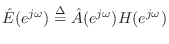
We now see precisely how the negative series inertance ![]() provides a
negative, frequency-dependent, length correction for the bore. From
(9.63),
the phase delay of
provides a
negative, frequency-dependent, length correction for the bore. From
(9.63),
the phase delay of ![]() can be computed as
can be computed as
In practice, it is common to combine all delay corrections into a single ``tuning allpass filter'' for the whole bore [428,207]. Whenever the desired allpass delay goes negative, we simply add a sample of delay to the desired allpass phase-delay and subtract it from the nearest delay. In other words, negative delays have to be ``pulled out'' of the allpass and used to shorten an adjacent interpolated delay line. Such delay lines are normally available in practical modeling situations.
Tonehole Filter Design
The tone-hole reflectance and transmittance must be converted to
discrete-time form for implementation in a digital waveguide model.
Figure 9.49 plots the responses of second-order discrete-time
filters designed to approximate the continuous-time magnitude and phase
characteristics of the reflectances for closed and open toneholes, as
carried out in [403,406]. These filter designs
assumed a tonehole of radius ![]() mm, minimum tonehole height
mm, minimum tonehole height
![]() mm, tonehole radius of curvature
mm, tonehole radius of curvature
![]() mm, and air column
radius
mm, and air column
radius ![]() mm. Since the measurements of Keefe do not extend to 5
kHz, the continuous-time responses in the figures are extrapolated above
this limit. Correspondingly, the filter designs were weighted to produce
best results below 5 kHz.
mm. Since the measurements of Keefe do not extend to 5
kHz, the continuous-time responses in the figures are extrapolated above
this limit. Correspondingly, the filter designs were weighted to produce
best results below 5 kHz.
The closed-hole filter design was carried out using weighted ![]() equation-error minimization [428, p. 47], i.e., by minimizing
equation-error minimization [428, p. 47], i.e., by minimizing
![]() , where
, where ![]() is the weighting
function,
is the weighting
function,
![]() is the desired frequency response,
is the desired frequency response, ![]() denotes
discrete-time radian frequency, and the designed filter response is
denotes
discrete-time radian frequency, and the designed filter response is
![]() . Note that both phase and magnitude are
matched by equation-error minimization, and this error criterion is used
extensively in the field of system identification [288]
due to its ability to design optimal IIR filters via quadratic
minimization. In the spirit of the well-known Steiglitz-McBride algorithm
[287], equation-error minimization can be iterated,
setting the weighting function at iteration
. Note that both phase and magnitude are
matched by equation-error minimization, and this error criterion is used
extensively in the field of system identification [288]
due to its ability to design optimal IIR filters via quadratic
minimization. In the spirit of the well-known Steiglitz-McBride algorithm
[287], equation-error minimization can be iterated,
setting the weighting function at iteration ![]() to the inverse of the
inherent weighting
to the inverse of the
inherent weighting
![]() of the previous iteration, i.e.,
of the previous iteration, i.e.,
![]() . However, for this study, the weighting was used only to
increase accuracy at low frequencies relative to high frequencies.
Weighted equation-error minimization is implemented in the matlab function
invfreqz() (§8.6.4).
. However, for this study, the weighting was used only to
increase accuracy at low frequencies relative to high frequencies.
Weighted equation-error minimization is implemented in the matlab function
invfreqz() (§8.6.4).
The open-hole discrete-time filter was designed using Kopec's method [297], [428, p. 46] in conjunction with weighted equation-error minimization. Kopec's method is based on linear prediction:
- Given a desired complex frequency response
 , compute an
allpole model
, compute an
allpole model
 using linear prediction
- Compute the error spectrum
 .
.
- Compute an allpole model
 for
for
 by
minimizing
by
minimizing
![\includegraphics[width=\twidth]{eps/twoptfilts}](http://www.dsprelated.com/josimages_new/pasp/img2522.png) |
The reasonably close match in both phase and magnitude by second-order filters indicates that there is in fact only one important tonehole resonance and/or anti-resonance within the audio band, and that the measured frequency responses can be modeled with very high audio accuracy using only second-order filters.
Figure 9.50 plots the reflection function calculated for a six-hole flute bore, as described in [240].
![\includegraphics[width=\twidth]{eps/gtwoport}](http://www.dsprelated.com/josimages_new/pasp/img2523.png) |
The Tonehole as a Two-Port Loaded Junction
It seems reasonable to expect that the tonehole should be
representable as a load along a waveguide bore model, thus
creating a loaded two-port junction with two identical bore ports on
either side of the tonehole. From the relations for the loaded
parallel junction (C.101), in the two-port case
with
![]() , and considering pressure waves rather than force
waves, we have
, and considering pressure waves rather than force
waves, we have
| (10.63) | |||
| (10.64) | |||
| (10.65) |
Thus, the loaded two-port junction can be implemented in ``one-filter form'' as shown in Fig. 9.48 with

Each series impedance ![]() in the split-T model of
Fig. 9.43 can be modeled as a series waveguide
junction with a load of
in the split-T model of
Fig. 9.43 can be modeled as a series waveguide
junction with a load of ![]() . To see this, set the transmission
matrix parameters in (9.55) to the values
. To see this, set the transmission
matrix parameters in (9.55) to the values
![]() ,
,
![]() , and
, and ![]() from (9.51) to get
from (9.51) to get
| (10.66) |
where
| (10.67) |
Next we convert pressure to velocity using
| (10.68) |
Finally, we toggle the reference direction of port 2 (the ``current'' arrow for
| (10.69) |
where
Next Section:
Bowed Strings
Previous Section:
Piano Synthesis


