


Biased Sample Autocorrelation
The sample autocorrelation defined in (6.6) is not quite
the same as the autocorrelation function for infinitely long
discrete-time sequences defined in §2.3.6,
viz.,
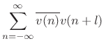
where the signal
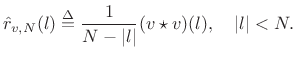
Thus,
![$\displaystyle (v\star v)(l) = \left\{\begin{array}{ll} (N-\left\vert l\right\vert) \hat{r}_{v,N}(l), & l=0,\pm1,\pm2,\ldots,\pm (N-1) \\ [5pt] 0, & \vert l\vert\geq N. \\ \end{array} \right. \protect$](http://www.dsprelated.com/josimages_new/sasp2/img1137.png)
It is common in practice to retain the implicit Bartlett (triangular) weighting in the sample autocorrelation. It merely corresponds to smoothing of the power spectrum (or cross-spectrum) with the
The left column of Fig.6.1 in fact shows the Bartlett-biased sample autocorrelation. When the bias is removed, the autocorrelation appears noisier at higher lags (near the endpoints of the plot).
Next Section:
Smoothed Power Spectral Density
Previous Section:
Sample Power Spectral Density


