Constant-Overlap-Add (COLA) Cases

Chapter Contents:

Search Spectral Audio Signal Processing

Book Index | Global Index

Would you like to be notified by email when Julius Orion Smith III publishes a new entry into his blog?

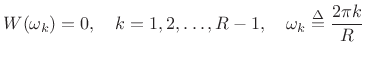
Weak COLA: Window transform has zeros at frame-rate harmonics:

$\displaystyle W(\omega_k) = 0, \quad k = 1,2, \dots, R-1, \quad \omega_k \isdef \frac{2\pi k}{R}$
- Perfect OLA reconstruction
- Relies on aliasing cancellation in frequency domain
- Aliasing cancellation is disturbed by spectral modifications
- See Portnoff for further details
Strong COLA: Window transform is bandlimited consistent with downsampling by the frame rate:

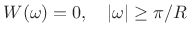
$\displaystyle W(\omega) = 0, \quad \vert\omega\vert \geq \pi/R$
- Perfect OLA reconstruction
- No aliasing
- better for spectral modifications
- Time-domain window infinitely long in ideal case

written by Julius Orion Smith III
Julius Smith's background is in electrical engineering (BS Rice 1975, PhD Stanford 1983). He is presently Professor of Music and Associate Professor (by courtesy) of Electrical Engineering at Stanford's Center for Computer Research in Music and Acoustics (CCRMA), teaching courses and pursuing research related to signal processing applied to music and audio systems. See http://ccrma.stanford.edu/~jos/ for details.

Sign in