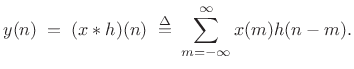
Convolution of Short Signals

figure[htbp]

Figure 7.1 illustrates the conceptual operation of filtering an input signal by a filter with impulse-response to produce an output signal . By the convolution theorem for DTFTs (§2.3.5),

or,

where and are arbitrary real or complex sequences, and and are the DTFTs of and , respectively. The convolution of and is defined by

In practice, we always use the DFT (preferably the FFT) in place of the DTFT, in which case we may write

where now (length complex sequences). It is important to remember that the specific form of convolution implied in the DFT case is cyclic (also called circular) convolution [248]:

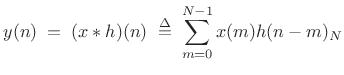
where means `` modulo .''

Another way to look at convolution is as the inner product of , and , where , i.e.,

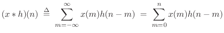
This form describes graphical convolution in which the output sample at time is computed as an inner product of the impulse response after flipping it about time 0 and shifting time 0 to time . See [248, p. 105] for an illustration of graphical convolution.

---

Subsections

• Cyclic FFT Convolution
• Acyclic FFT Convolution
  • Acyclic Convolution in Matlab or Octave
  • Pictorial View of Acyclic Convolution
  
  
• Acyclic FFT Convolution in Matlab or Octave
• FFT versus Direct Convolution
  • Audio FIR Filters
  • Example 1: Low-Pass Filtering by FFT Convolution
  • Example 2: Time Domain Aliasing

---

Previous: Overlap-Add (OLA) STFT Processing
Next: Cyclic FFT Convolution

Order a Hardcopy of Spectral Audio Signal Processing

---

About the Author: Julius Orion Smith III
Julius Smith's background is in electrical engineering (BS Rice 1975, PhD Stanford 1983). He is presently Professor of Music and Associate Professor (by courtesy) of Electrical Engineering at Stanford's Center for Computer Research in Music and Acoustics (CCRMA), teaching courses and pursuing research related to signal processing applied to music and audio systems. See http://ccrma.stanford.edu/~jos/ for details.