


Dual Views of the Short Time Fourier Transform (STFT)
In the overlap-add formulation of Chapter 8, we used a
hopping window to extract time-limited signals to which we
applied the DFT. Assuming for the moment that the hop size ![]() (the ``sliding DFT''), we have
(the ``sliding DFT''), we have
![$\displaystyle \zbox {X_m(\omega_k) = \sum_{n=-\infty}^\infty [w(n-m) x(n)] e^{-j\omega_k n}.} \protect$](http://www.dsprelated.com/josimages_new/sasp2/img1535.png)
This is the usual definition of the Short-Time Fourier Transform (STFT) (§7.1). In this chapter, we will look at the STFT from two different points of view: the OverLap-Add (OLA) and Filter-Bank Summation (FBS) points of view. We will show that one is the Fourier dual of the other [9]. Next we will explore some implications of the filter-bank point of view and obtain some useful insights. Finally, some applications are considered.
Overlap-Add (OLA) Interpretation of the STFT
In the OLA interpretation of the STFT, we apply a time-shifted window
![]() to our signal
to our signal ![]() , selecting data near time
, selecting data near time ![]() , and
compute the Fourier-transform to obtain the spectrum of the
, and
compute the Fourier-transform to obtain the spectrum of the ![]() th
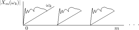
frame. As shown in Fig.9.1, the STFT is viewed as a
time-ordered sequence of spectra, one per frame, with the
frames overlapping in time.
th
frame. As shown in Fig.9.1, the STFT is viewed as a
time-ordered sequence of spectra, one per frame, with the
frames overlapping in time.
Filter-Bank Summation (FBS) Interpretation of the STFT
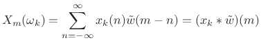
We can group the terms in the STFT definition differently to obtain
the filter-bank interpretation:
![$\displaystyle \sum_{n=-\infty}^\infty \underbrace{[ x(n)e^{-j\omega_k n}]}_{x_k(n)} w(n-m)$](http://www.dsprelated.com/josimages_new/sasp2/img1538.png)
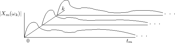
As will be explained further below (and illustrated further in Figures 9.3, 9.4, and 9.5), under the filter-bank interpretation, the spectrum of
Expanding on the previous paragraph, the STFT (9.2) is computed by the following operations:
- Frequency-shift
 by
by  to get
 .
.
- Convolve
 with
with
 to get
 :
:
(10.3)
Note that the STFT analysis window ![]() is now interpreted as (the flip
of) a lowpass-filter impulse response. Since the analysis window
is now interpreted as (the flip
of) a lowpass-filter impulse response. Since the analysis window ![]() in the STFT is typically symmetric, we usually have
in the STFT is typically symmetric, we usually have
![]() .
This filter is effectively frequency-shifted to provide each channel
bandpass filter. If the cut-off frequency of the window transform is
.
This filter is effectively frequency-shifted to provide each channel
bandpass filter. If the cut-off frequency of the window transform is
![]() (typically half a main-lobe width), then each channel
signal can be downsampled significantly. This downsampling factor is
the FBS counterpart of the hop size
(typically half a main-lobe width), then each channel
signal can be downsampled significantly. This downsampling factor is
the FBS counterpart of the hop size ![]() in the OLA context.
in the OLA context.
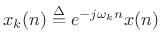
Figure 9.3 illustrates the filter-bank interpretation for ![]() (the ``sliding STFT''). The input signal
(the ``sliding STFT''). The input signal ![]() is frequency-shifted
by a different amount for each channel and lowpass filtered by the
(flipped) window.
is frequency-shifted
by a different amount for each channel and lowpass filtered by the
(flipped) window.
![\begin{psfrags}
% latex2html id marker 23871\psfrag{w}{\Large$\protect\hbox{\sc Flip}(w)$}\psfrag{x(n)}{\LARGE$x(n)$}\psfrag{X0}{\LARGE$X_n(\omega_{\scriptscriptstyle 0}$)}\psfrag{X1}{\LARGE$X_n(\omega_{\scriptscriptstyle 1}$)}\psfrag{XNm1}{\LARGE$X_n(\omega_{\scriptscriptstyle {N}-1})$}\psfrag{ejw0}{\huge$e^{-j\omega_{\scriptscriptstyle 0}n}$}\psfrag{ejw1}{\huge$e^{-j\omega_{\scriptscriptstyle 1}n}$}\psfrag{ejwNm1}{\huge$e^{-j\omega_{\scriptscriptstyle {N-1}}n}$}\psfrag{dR}{\LARGE$\downarrow R$}\psfrag{X}{\LARGE$\times$}\begin{figure}[htbp]
\includegraphics[width=3in]{eps/fbs1}
\caption{Sliding STFT analysis filter bank.
The $k$th channel of the filter bank computes
$X_n(\omega_k)=(x_k\ast \hbox{\sc Flip}{w})(n)$, where $x_k(n)\isdeftext
x(n)\exp(-j\omega_k n)$.
}
\end{figure}
\end{psfrags}](http://www.dsprelated.com/josimages_new/sasp2/img1552.png)
FBS and Perfect Reconstruction
An important property of the STFT established in Chapter 8 is that it is exactly invertible when the analysis window satisfies the constant-overlap-add constraint. That is, neglecting numerical round-off error, the inverse STFT reproduces the original input signal exactly. This is called the perfect reconstruction property of the STFT, and modern filter banks are usually designed with this property in mind [287].
In the OLA processors of Chapter 8, perfect reconstruction was
assured by using FFT analysis windows ![]() having the
Constant-Overlap-Add (COLA) property at the particular hop-size
having the
Constant-Overlap-Add (COLA) property at the particular hop-size
![]() used (see §8.2.1).
used (see §8.2.1).
In the Filter Bank Summation (FBS) interpretation of the STFT
(Eq.![]() (9.1)), it is the analysis filter-bank frequency
responses
(9.1)), it is the analysis filter-bank frequency
responses
![]() that are constrained to be COLA. We
will take a look at this more closely below.
that are constrained to be COLA. We
will take a look at this more closely below.
Next Section:
STFT Filter Bank
Previous Section:
Review of Zero Padding


