


Filtered White Noise
When a white-noise sequence is filtered, successive samples generally become correlated.7.8 Some of these filtered-white-noise signals have names:
- pink noise: Filter amplitude response
 is proportional to
 ; PSD
; PSD
 (``1/f noise'' -- ``equal-loudness noise'')
- brown noise: Filter amplitude response
is proportional to
 ; PSD
; PSD
 (``Brownian motion'' -- ``Wiener process'' -- ``random increments'')
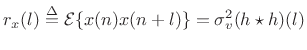
In the preceding sections, we have looked at two ways of analyzing noise: the sample autocorrelation function in the time or ``lag'' domain, and the sample power spectral density (PSD) in the frequency domain. We now look at these two representations for the case of filtered noise.
Let ![]() denote a length
denote a length ![]() sequence we wish to analyze. Then the
Bartlett-windowed acyclic sample autocorrelation of
sequence we wish to analyze. Then the
Bartlett-windowed acyclic sample autocorrelation of ![]() is
is ![]() ,
and the corresponding smoothed sample PSD is
,
and the corresponding smoothed sample PSD is
![]() (§6.7, §2.3.6).
(§6.7, §2.3.6).
For filtered white noise, we can write ![]() as a convolution of white
noise
as a convolution of white
noise ![]() and some impulse response
and some impulse response ![]() :
:
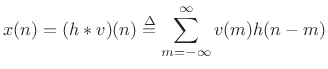 |
(7.29) |
The DTFT of
| (7.30) |
so that
since
![]() for white noise.
Thus, we have derived that the autocorrelation of filtered white noise
is proportional to the autocorrelation of the impulse response times
the variance of the driving white noise.
for white noise.
Thus, we have derived that the autocorrelation of filtered white noise
is proportional to the autocorrelation of the impulse response times
the variance of the driving white noise.
Let's try to pin this down more precisely and find the proportionality
constant. As the number ![]() of observed samples of
of observed samples of
![]() goes to infinity, the length-
goes to infinity, the length-![]() Bartlett-window bias
Bartlett-window bias ![]() in the autocorrelation
in the autocorrelation ![]() converges to a constant scale factor
converges to a constant scale factor
![]() at lags such that
at lags such that ![]() . Therefore, the unbiased
autocorrelation can be expressed as
. Therefore, the unbiased
autocorrelation can be expressed as
 |
(7.31) |
In the limit, we obtain
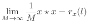 |
(7.32) |
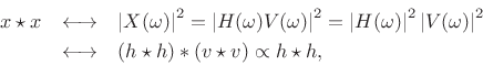
In the frequency domain we therefore have
![\begin{eqnarray*}
S_x(\omega) &=&
\lim_{M\to \infty}\frac{1}{M}\vert X(\omega)\vert^2 \;=\;
% = \frac{1}{M}\vert H(\omega)\,V(\omega)\vert^2
\vert H(\omega)\vert^2 \cdot \lim_{M\to \infty} \frac{\vert V(\omega)\vert^2}{M} \\ [5pt]
&=&
\vert H(\omega)\vert^2 S_v(\omega) \;=\;
\vert H(\omega)\vert^2\sigma_v^2 \;\longleftrightarrow\;
(h\star h) \sigma_v^2 .
\end{eqnarray*}](http://www.dsprelated.com/josimages_new/sasp2/img1198.png)
In summary, the autocorrelation of filtered white noise ![]() is
is
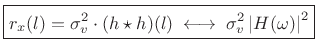 |
(7.33) |
where
In words, the true autocorrelation of filtered white noise equals the autocorrelation of the filter's impulse response times the white-noise variance. (The filter is of course assumed LTI and stable.) In the frequency domain, we have that the true power spectral density of filtered white noise is the squared-magnitude frequency response of the filter scaled by the white-noise variance.
For finite number of observed samples of a filtered white noise
process, we may say that the sample autocorrelation of filtered white
noise is given by the autocorrelation of the filter's impulse response
convolved with the sample autocorrelation of the driving white-noise
sequence. For lags ![]() much less than the number of observed samples
much less than the number of observed samples
![]() , the driver sample autocorrelation approaches an impulse scaled by
the white-noise variance. In the frequency domain, we have that the
sample PSD of filtered white noise is the squared-magnitude frequency
response of the filter
, the driver sample autocorrelation approaches an impulse scaled by
the white-noise variance. In the frequency domain, we have that the
sample PSD of filtered white noise is the squared-magnitude frequency
response of the filter
![]() scaled by a sample PSD of the
driving noise.
scaled by a sample PSD of the
driving noise.
We reiterate that every stationary random process may be defined, for our purposes, as filtered white noise.7.9 As we see from the above, all correlation information is embodied in the filter used.
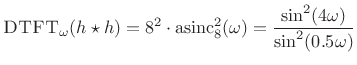
Example: FIR-Filtered White Noise
Let's estimate the autocorrelation and power spectral density of the ``moving average'' (MA) process
| (7.34) |
where
Since
![]() ,
,
| (7.35) |
for nonnegative lags (
![$\displaystyle (h\star h)(l) = \left\{\begin{array}{ll} 8-l, & \vert l\vert<8 \\ [5pt] 0, & \vert l\vert\ge 8. \\ \end{array} \right.$](http://www.dsprelated.com/josimages_new/sasp2/img1206.png) |
(7.36) |
Thus, the autocorrelation of
 |
(7.37) |
The true power spectral density (PSD) is then
 |
(7.38) |
Figure 6.3 shows a collection of measured autocorrelations together with their associated smoothed-PSD estimates.
![\includegraphics[width=\twidth]{eps/tcolored}](http://www.dsprelated.com/josimages_new/sasp2/img1209.png) |
Example: Synthesis of 1/F Noise (Pink Noise)
Pink noise7.10 or
``1/f noise'' is an interesting case because it occurs often in nature
[294],7.11is often preferred by composers of computer music, and there is no
exact (rational, finite-order) filter which can produce it from
white noise. This is because the ideal amplitude response of
the filter must be proportional to the irrational function
![]() , where
, where ![]() denotes frequency in Hz. However, it is easy
enough to generate pink noise to any desired degree of approximation,
including perceptually exact.
denotes frequency in Hz. However, it is easy
enough to generate pink noise to any desired degree of approximation,
including perceptually exact.
The following Matlab/Octave code generates pretty good pink noise:
Nx = 2^16;  % number of samples to synthesize
B = [0.049922035 -0.095993537 0.050612699 -0.004408786];
A = [1 -2.494956002   2.017265875  -0.522189400];
nT60 = round(log(1000)/(1-max(abs(roots(A))))); % T60 est.
v = randn(1,Nx+nT60); % Gaussian white noise: N(0,1)
x = filter(B,A,v);    % Apply 1/F roll-off to PSD
x = x(nT60+1:end);    % Skip transient response
In the next section, we will analyze the noise produced by the above matlab and verify that its power spectrum rolls off at approximately 3 dB per octave.
Example: Pink Noise Analysis
Let's test the pink noise generation algorithm presented in
§6.14.2. We might want to know, for example, does the power
spectral density really roll off as ![]() ? Obviously such a shape
cannot extend all the way to dc, so how far does it go? Does it go
far enough to be declared ``perceptually equivalent'' to ideal 1/f
noise? Can we get by with fewer bits in the filter coefficients?
Questions like these can be answered by estimating the power spectral
density of the noise generator output.
? Obviously such a shape
cannot extend all the way to dc, so how far does it go? Does it go
far enough to be declared ``perceptually equivalent'' to ideal 1/f
noise? Can we get by with fewer bits in the filter coefficients?
Questions like these can be answered by estimating the power spectral
density of the noise generator output.
Figure 6.4 shows a single periodogram of the generated pink noise, and Figure 6.5 shows an averaged periodogram (Welch's method of smoothed power spectral density estimation). Also shown in each log-log plot is the true 1/f roll-off line. We see that indeed a single periodogram is quite random, although the overall trend is what we expect. The more stable smoothed PSD estimate from Welch's method (averaged periodograms) gives us much more confidence that the noise generator makes high quality 1/f noise.
Note that we do not have to test for stationarity in this example, because we know the signal was generated by LTI filtering of white noise. (We trust the randn function in Matlab and Octave to generate stationary white noise.)
![\includegraphics[width=\twidth]{eps/noisepr}](http://www.dsprelated.com/josimages_new/sasp2/img1210.png)
![\includegraphics[width=\twidth]{eps/noisep}](http://www.dsprelated.com/josimages_new/sasp2/img1211.png)
Next Section:
Processing Gain
Previous Section:
Welch's Method with Windows


