


Generalized Hamming Window Family
The generalized Hamming window family is constructed by multiplying a rectangular window by one period of a cosine. The benefit of the cosine tapering is lower side-lobes. The price for this benefit is that the main-lobe doubles in width. Two well known members of the generalized Hamming family are the Hann and Hamming windows, defined below.
The basic idea of the generalized Hamming family can be seen in the
frequency-domain picture of Fig.3.8. The center dotted
waveform is the aliased sinc function
![]() (scaled rectangular window transform). The
other two dotted waveforms are scaled shifts of the same function,
(scaled rectangular window transform). The
other two dotted waveforms are scaled shifts of the same function,
![]() . The sum of all three dotted waveforms gives
the solid line. We see that
. The sum of all three dotted waveforms gives
the solid line. We see that
- there is some cancellation of the side lobes, and
- the width of the main lobe is doubled.
![\includegraphics[width=3in]{eps/shiftedSincs}](http://www.dsprelated.com/josimages_new/sasp2/img356.png) |
In terms of the rectangular window transform
![]() (the zero-phase, unit-amplitude case), this
can be written as
(the zero-phase, unit-amplitude case), this
can be written as
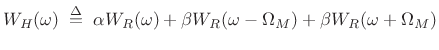 |
(4.15) |
where
Using the shift theorem (§2.3.4), we can take the inverse transform of the above equation to obtain
| (4.16) |
or,
![$\displaystyle \zbox {w_H(n) = w_R(n) \left[ \alpha + 2 \beta \cos \left( \frac{2 \pi n}{M} \right) \right].} \protect$](http://www.dsprelated.com/josimages_new/sasp2/img361.png)
Choosing various parameters for ![]() and
and ![]() result in
different windows in the generalized Hamming family, some of which
have names.
result in
different windows in the generalized Hamming family, some of which
have names.
Hann or Hanning or Raised Cosine
The Hann window (or hanning or raised-cosine
window) is defined based on the settings
![]() and
and ![]() in
(3.17):
in
(3.17):
![$\displaystyle w_H(n)=w_R(n) \left[ \frac{1}{2} + \frac{1}{2} \cos( \Omega_M n) \right] = w_R(n) \cos^2\left(\frac{\Omega_M}{2} n\right) \protect$](http://www.dsprelated.com/josimages_new/sasp2/img362.png)
where
The Hann window and its transform appear in Fig.3.9. The
Hann window can be seen as one period of a cosine ``raised'' so that
its negative peaks just touch zero (hence the alternate name ``raised cosine'').
Since it reaches zero at its endpoints with zero slope, the
discontinuity leaving the window is in the second derivative, or the
third term of its Taylor series expansion at an endpoint. As a
result, the side lobes roll off approximately 18 dB per octave. In
addition to the greatly accelerated roll-off rate, the first side lobe
has dropped from ![]() dB (rectangular-window case) down to
dB (rectangular-window case) down to ![]() dB. The main-lobe width is of course double that of the rectangular
window. For Fig.3.9, the window was computed in Matlab
as hanning(21). Therefore, it is the variant that places the
zero endpoints one-half sample to the left and right of the outermost
window samples (see next section).
dB. The main-lobe width is of course double that of the rectangular
window. For Fig.3.9, the window was computed in Matlab
as hanning(21). Therefore, it is the variant that places the
zero endpoints one-half sample to the left and right of the outermost
window samples (see next section).
![\includegraphics[width=4in]{eps/hanningWindow}](http://www.dsprelated.com/josimages_new/sasp2/img365.png)
Matlab for the Hann Window
In matlab, a length ![]() Hann window is designed by the statement
Hann window is designed by the statement
w = hanning(M);which, in Matlab only is equivalent to
w = .5*(1 - cos(2*pi*(1:M)'/(M+1)));For
>> hanning(3)
ans =
     0.5
     1
     0.5
Note the curious use of M+1 in the denominator instead of
M as we would expect from the family definition in
(3.17). This perturbation serves to avoid using zero samples in
the window itself. (Why bother to multiply explicitly by zero?) Thus,
the Hann window as returned by Matlab hanning function
reaches zero one sample beyond the endpoints to the left and right.
The minus sign, which differs from (3.18), serves to make the
window causal instead of zero phase.
The Matlab Signal Processing Toolbox also includes a hann function which is defined to include the zeros at the window endpoints. For example,
>> hann(3)
ans =
     0
     1
     0
This case is equivalent to the following matlab expression:w = .5*(1 - cos(2*pi*(0:M-1)'/(M-1)));The use of
In Matlab, both hann(3,'periodic') and hanning(3,'periodic') produce the following window:
>> hann(3,'periodic')
ans =
     0
     0.75
     0.75
This case is equivalent to w = .5*(1 - cos(2*pi*(0:M-1)'/M));which agrees (finally) with definition (3.18). We see that in this case, the left zero endpoint is included in the window, while the one on the right lies one sample outside to the right. In general, the 'periodic' window option asks for a window that can be overlapped and added to itself at certain time displacements (
In Octave, both the hann and hanning functions include the endpoint zeros.
In practical applications, it is safest to write your own window functions in the matlab language in order to ensure portability and consistency. After all, they are typically only one line of code!
In comparing window properties below, we will speak of the Hann window
as having a main-lobe width equal to ![]() , and a side-lobe
width
, and a side-lobe
width ![]() , even though in practice they may really be
, even though in practice they may really be
![]() and
and
![]() , respectively, as illustrated
above. These remarks apply to all windows in the generalized Hamming
family, as well as the Blackman-Harris family introduced in
§3.3 below.
, respectively, as illustrated
above. These remarks apply to all windows in the generalized Hamming
family, as well as the Blackman-Harris family introduced in
§3.3 below.
Summary of Hann window properties:
- Main lobe is
 wide,
wide,
- First side lobe at -31dB
- Side lobes roll off approximately
 dB per octave
Hamming Window
The Hamming window is determined by choosing ![]() in
(3.17) (with
in
(3.17) (with
![]() ) to cancel the largest side lobe
[101].4.4 Doing this results in the values
) to cancel the largest side lobe
[101].4.4 Doing this results in the values
![\begin{eqnarray*}
\alpha &=& \frac{25}{46} \approx 0.54\\ [5pt]
\beta &=& \frac{1-\alpha}{2} \approx 0.23.
\end{eqnarray*}](http://www.dsprelated.com/josimages_new/sasp2/img375.png)
The peak side-lobe level is approximately ![]() dB for the Hamming
window [101].4.5 It happens that this
choice is very close to that which minimizes peak side-lobe level
(down to
dB for the Hamming
window [101].4.5 It happens that this
choice is very close to that which minimizes peak side-lobe level
(down to ![]() dB--the lowest possible within the generalized
Hamming family) [196]:
dB--the lowest possible within the generalized
Hamming family) [196]:
| (4.19) |
Since rounding the optimal
![\includegraphics[width=\twidth]{eps/hammingWindow}](http://www.dsprelated.com/josimages_new/sasp2/img381.png)
The Hamming window and its DTFT magnitude are shown in
Fig.3.10. Like the Hann window, the Hamming window is
also one period of a raised cosine. However, the cosine is raised so
high that its negative peaks are above zero, and the window has
a discontinuity in amplitude at its endpoints (stepping
discontinuously from 0.08 to 0). This makes the side-lobe roll-off
rate very slow (asymptotically ![]() dB/octave). On the other hand,
the worst-case side lobe plummets to
dB/octave). On the other hand,
the worst-case side lobe plummets to ![]() dB,4.6which is the purpose of the Hamming window. This is 10 dB better than
the Hann case of Fig.3.9 and 28 dB better than the
rectangular window. The main lobe is approximately
dB,4.6which is the purpose of the Hamming window. This is 10 dB better than
the Hann case of Fig.3.9 and 28 dB better than the
rectangular window. The main lobe is approximately ![]() wide,
as is the case for all members of the generalized Hamming family
(
wide,
as is the case for all members of the generalized Hamming family
(
![]() ).
).
Due to the step discontinuity at the window boundaries, we expect a
spectral envelope which is an aliased version of a ![]() dB per octave
(i.e., a
dB per octave
(i.e., a ![]() roll-off is converted to a ``cosecant roll-off'' by
aliasing, as derived in §3.1 and illustrated in
Fig.3.6). However, for the Hamming window, the
side-lobes nearest the main lobe have been strongly shaped by the
optimization. As a result, the nearly
roll-off is converted to a ``cosecant roll-off'' by
aliasing, as derived in §3.1 and illustrated in
Fig.3.6). However, for the Hamming window, the
side-lobes nearest the main lobe have been strongly shaped by the
optimization. As a result, the nearly ![]() dB per octave roll-off
occurs only over an interior interval of the spectrum, well between
the main lobe and half the sampling rate. This is easier to see for a
larger
dB per octave roll-off
occurs only over an interior interval of the spectrum, well between
the main lobe and half the sampling rate. This is easier to see for a
larger ![]() , as shown in
Fig.3.11, since then the optimized side-lobes nearest
the main lobe occupy a smaller frequency interval about the main
lobe.
, as shown in
Fig.3.11, since then the optimized side-lobes nearest
the main lobe occupy a smaller frequency interval about the main
lobe.
![\includegraphics[width=\twidth]{eps/hammingWindowLong}](http://www.dsprelated.com/josimages_new/sasp2/img384.png)
Since the Hamming window side-lobe level is more than 40 dB down, it
is often a good choice for ``1% accurate systems,'' such as 8-bit
audio signal processing systems. This is because there is rarely any
reason to require the window side lobes to lie far below the signal
quantization noise floor. The Hamming window has been extensively
used in telephone communications signal processing wherein 8-bit
CODECs were standard for many decades (albeit ![]() -law encoded).
For higher quality audio signal processing, higher quality windows may
be required, particularly when those windows act as lowpass filters
(as developed in Chapter 9).
-law encoded).
For higher quality audio signal processing, higher quality windows may
be required, particularly when those windows act as lowpass filters
(as developed in Chapter 9).
Matlab for the Hamming Window
In matlab, a length ![]() Hamming window is designed by the statement
Hamming window is designed by the statement
w = hamming(M);which is equivalent to
w = .54 - .46*cos(2*pi*(0:M-1)'/(M-1));Note that M-1 is used in the denominator rather than M+1 as in the Hann window case. Since the Hamming window cannot reach zero for any choice of samples of the defining raised cosine, it makes sense not to have M+1 here. Using M-1 (instead of M) provides that the returned window is symmetric, which is usually desired. However, we will learn later that there are times when M is really needed in the denominator (such as when the window is being used successively over time in an overlap-add scheme, in which case the sum of overlapping windows must be constant).
The hamming function in the Matlab Signal Processing Tool
Box has an optional argument 'periodic' which effectively
uses ![]() instead of
instead of ![]() . The default case is 'symmetric'.
The following examples should help clarify the difference:
. The default case is 'symmetric'.
The following examples should help clarify the difference:
>> hamming(3) % same in Matlab and Octave
ans =
    0.0800
    1.0000
    0.0800
>> hamming(3,'symmetric') % Matlab only
ans =
    0.0800
    1.0000
    0.0800
>> hamming(3,'periodic') % Matlab only
ans =
    0.0800
    0.7700
    0.7700
>> hamming(4) % same in Matlab and Octave
ans =
    0.0800
    0.7700
    0.7700
    0.0800
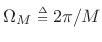
Summary of Generalized Hamming Windows
Definition:
![$\displaystyle w_H(n) = w_R(n) \left[ \alpha + 2 \beta \cos \left( \Omega_M n \right) \right], \quad n \in {\bf Z}, \; \Omega_M \isdef \frac{2 \pi}{M}$](http://www.dsprelated.com/josimages_new/sasp2/img386.png) |
(4.20) |
where
![$\displaystyle w_R(n) \isdefs \left\{\begin{array}{ll} 1, & \left\vert n\right\vert\leq\frac{M-1}{2} \\ [5pt] 0, & \hbox{otherwise} \\ \end{array} \right.$](http://www.dsprelated.com/josimages_new/sasp2/img387.png) |
(4.21) |
Transform:
 |
(4.22) |
where
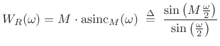 |
(4.23) |
Common Properties
- Rectangular + scaled-cosine window
- Cosine has one period across the window
- Symmetric (
 zero or linear phase)
- Positive (by convention on
 and
and  )
)
- Main lobe is
radians per sample wide, where

- Zero-crossings (``notches'') in window transform at intervals
of
 outside of main lobe
Figure 3.12 compares the window transforms for the rectangular, Hann, and Hamming windows. Note how the Hann window has the fastest roll-off while the Hamming window is closest to being equal-ripple. The rectangular window has the narrowest main lobe.
![\includegraphics[width=\twidth]{eps/RectHannHamm}](http://www.dsprelated.com/josimages_new/sasp2/img392.png)
Rectangular window properties:
- Abrupt transition from 1 to 0 at the window endpoints
- Roll-off is asymptotically
 dB per octave (as
 )
)
- First side lobe is
 dB relative to main-lobe peak
Hann window properties:
- Smooth transition to zero at window endpoints
- Roll-off is asymptotically -18 dB per octave
- First side lobe is
 dB relative to main-lobe peak
Hamming window properties:
- Discontinuous ``slam to zero'' at endpoints
- Roll-off is asymptotically -6 dB per octave
- Side lobes are closer to ``equal ripple''
- First side lobe is
 dB down =
  dB better than
Hann4.7
dB better than
Hann4.7
The MLT Sine Window
The modulated lapped transform (MLT) [160] uses the sine window, defined by
![$\displaystyle w(n) = \sin\left[\left(n+\frac{1}{2}\right)\frac{\pi}{2M}\right], \quad n=0,1,2,\ldots,2M-1\,.$](http://www.dsprelated.com/josimages_new/sasp2/img398.png) |
(4.24) |
The sine window is used in MPEG-1, Layer 3 (MP3 format), MPEG-2 AAC, and MPEG-4 [200].
Properties:
- Side lobes 24 dB down
- Asymptotically optimal coding gain [159]
- Zero-phase-window transform (``truncated cosine window'')
has smallest moment of inertia over all windows [202]:
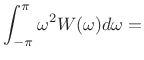 min
min(4.25)
Note that in perceptual audio coding systems, there is both an
analysis window and a synthesis window. That is, the
sine window is deployed twice, first when encoding the signal,
and second when decoding. As a result, the sine window is
squared in practical usage, rendering it equivalent to a Hann
window (![]() ) in the final output signal (when there are no
spectral modifications).
) in the final output signal (when there are no
spectral modifications).
It is of great practical value that the second window application occurs after spectral modifications (such as spectral quantization); any distortions due to spectral modifications are tapered gracefully to zero by the synthesis window. Synthesis windows were introduced at least as early as 1980 [213,49], and they became practical for audio coding with the advent of time-domain aliasing cancellation (TDAC) [214]. The TDAC technique made it possible to use windows with 50% overlap without suffering a doubling of the number of samples in the short-time Fourier transform. TDAC was generalized to ``lapped orthogonal transforms'' (LOT) by Malvar [160]. The modulated lapped transform (MLT) is a variant of LOT used in conjunction with the modulated discrete cosine transform (MDCT) [160]. See also [287] and [291].
Next Section:
Blackman-Harris Window Family
Previous Section:
The Rectangular Window


