


Geometric Signal Theory
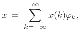
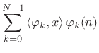
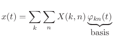
In general, signals can be expanded as a linear combination
of orthonormal basis signals ![]() [264]. In the
discrete-time case, this can be expressed as
[264]. In the
discrete-time case, this can be expressed as
where the coefficient of projection of
 |
(12.105) |
and the basis signals are orthonormal:
 |
(12.106) |
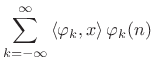
The signal expansion (11.104) can be interpreted geometrically as a sum of orthogonal projections of
![\includegraphics[width=0.5\twidth]{eps/proj}](http://www.dsprelated.com/josimages_new/sasp2/img2285.png)
A set of signals
![]() is said to be
a biorthogonal basis set if any signal
is said to be
a biorthogonal basis set if any signal ![]() can be represented
as
can be represented
as
 |
(12.107) |
where
The following examples illustrate the Hilbert space point of view for various familiar cases of the Fourier transform and STFT. A more detailed introduction appears in Book I [264].
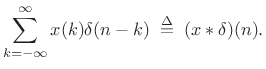
Natural Basis
The natural basis for a discrete-time signal ![]() is the set
of shifted impulses:
is the set
of shifted impulses:
![$\displaystyle \varphi_k \isdefs [\ldots, 0,\underbrace{1}_{k^{\hbox{\tiny th}}},0,\ldots],$](http://www.dsprelated.com/josimages_new/sasp2/img2291.png) |
(12.108) |
or,
 |
(12.109) |
for all integers
| (12.110) |
so that the expansion of
 |
(12.111) |
i.e.,
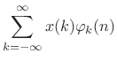 |
|||
 |
This expansion was used in Book II [263] to derive the impulse-response representation of an arbitrary linear, time-invariant filter.
Normalized DFT Basis for 
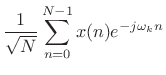
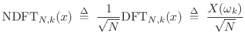
The Normalized Discrete Fourier Transform (NDFT) (introduced in
Book I [264]) projects the signal ![]() onto
onto ![]() discrete-time sinusoids of length
discrete-time sinusoids of length ![]() , where the sinusoids are
normalized to have unit
, where the sinusoids are
normalized to have unit ![]() norm:
norm:
 |
(12.112) |
and
 |
|||
 |
and the expansion of
 |
|||
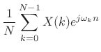 |
|||
for
Normalized Fourier Transform Basis
The Fourier transform projects a continuous-time signal ![]() onto an
infinite set of continuous-time complex sinusoids
onto an
infinite set of continuous-time complex sinusoids
![]() ,
for
,
for
![]() . These sinusoids all have infinite
. These sinusoids all have infinite ![]() norm, but a simple normalization by
norm, but a simple normalization by
![]() can be chosen so
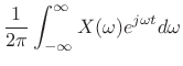
that the inverse Fourier transform has the desired form of a
superposition of projections:
can be chosen so
that the inverse Fourier transform has the desired form of a
superposition of projections:
 |
(12.113) |
 |
|||
 |
|||
 |
|||
 |
|||
Normalized DTFT Basis
The Discrete Time Fourier Transform (DTFT) is similar to the Fourier transform case:
![$\displaystyle \varphi _\omega (n) \isdef e^{j\omega n}/\sqrt{2\pi},\quad \omega \in (-\pi,\pi], \quad n\in (-\infty,\infty)$](http://www.dsprelated.com/josimages_new/sasp2/img2317.png) |
(12.114) |
The inner product
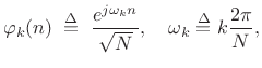
Normalized STFT Basis
The Short Time Fourier Transform (STFT) is defined as a time-ordered
sequence of DTFTs, and implemented in practice as a sequence of FFTs
(see §7.1). Thus, the signal basis functions are naturally
defined as the DFT-sinusoids multiplied by time-shifted windows,
suitably normalized for unit ![]() norm:
norm:
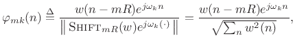 |
(12.115) |
![$\displaystyle \omega_k = \frac{2\pi k}{N}, \quad k \in [0,N-1], \quad n\in (-\infty,\infty),\quad w(n)\in{\cal R},$](http://www.dsprelated.com/josimages_new/sasp2/img2321.png) |
(12.116) |
and
When successive windows overlap (i.e., the hop size ![]() is less than
the window length
is less than
the window length ![]() ), the basis functions are not
orgthogonal. In this case, we may say that the basis set
is overcomplete.
), the basis functions are not
orgthogonal. In this case, we may say that the basis set
is overcomplete.
The basis signals are orthonormal when ![]() and the rectangular
window is used (
and the rectangular
window is used (![]() ). That is, two rectangularly windowed DFT
sinusoids are orthogonal when either the frequency bin-numbers or the
time frame-numbers differ, provided that the window length
). That is, two rectangularly windowed DFT
sinusoids are orthogonal when either the frequency bin-numbers or the
time frame-numbers differ, provided that the window length ![]() equals
the number of DFT frequencies
equals
the number of DFT frequencies ![]() (no zero padding). In other words,
we obtain an orthogonal basis set in the STFT when the hop size,
window length, and DFT length are all equal (in which case the
rectangular window must be used to retain the perfect-reconstruction
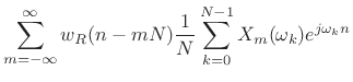
property). In this case, we can write
(no zero padding). In other words,
we obtain an orthogonal basis set in the STFT when the hop size,
window length, and DFT length are all equal (in which case the
rectangular window must be used to retain the perfect-reconstruction
property). In this case, we can write
| (12.117) |
i.e.,
![$\displaystyle \varphi_{mk}(n) = \left\{\begin{array}{ll} \frac{e^{j\omega_k n}}{\sqrt{N}}, & mN \leq n \leq (m+1)N-1 \\ [5pt] 0, & \mbox{otherwise.} \\ \end{array} \right.$](http://www.dsprelated.com/josimages_new/sasp2/img2324.png) |
(12.118) |
The coefficient of projection can be written
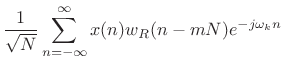 |
|||
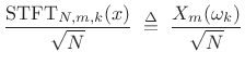 |
so that the signal expansion can be interpreted as
 |
|||
 |
|||
![$\displaystyle \sum_{m=-\infty}^{\infty}
\hbox{\sc Shift}_{mN,n}\left\{\hbox{\sc ZeroPad}_\infty\left[\hbox{DFT}_N^{-1}(X_m)\right]\right\}$](http://www.dsprelated.com/josimages_new/sasp2/img2331.png) |
|||
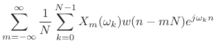
In the overcomplete case, we get a special case of weighted
overlap-add (§8.6):
|
|||
 |
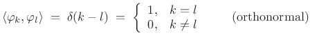
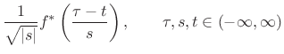
Continuous Wavelet Transform
In the present (Hilbert space) setting, we can now easily define the continuous wavelet transform in terms of its signal basis set:
 |
|||
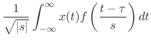 |
The parameter
![\includegraphics[width=0.8\twidth]{eps/wavelets}](http://www.dsprelated.com/josimages_new/sasp2/img2341.png)
The so-called admissibility condition for a mother wavelet
![]() is
is
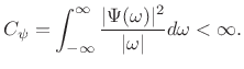
Given sufficient decay with
The Morlet wavelet is simply a Gaussian-windowed complex sinusoid:
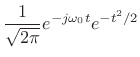 |
|||
The scale factor is chosen so that
| (12.119) |
In this case, we have
Since the scale parameter of a wavelet transform is analogous to frequency in a Fourier transform, a wavelet transform display is often called a scalogram, in analogy with an STFT ``spectrogram'' (discussed in §7.2).
When the mother wavelet can be interpreted as a windowed sinusoid (such as the Morlet wavelet), the wavelet transform can be interpreted as a constant-Q Fourier transform.12.5Before the theory of wavelets, constant-Q Fourier transforms (such as obtained from a classic third-octave filter bank) were not easy to invert, because the basis signals were not orthogonal. See Appendix E for related discussion.
Discrete Wavelet Transform
The discrete wavelet transform is a discrete-time,
discrete-frequency counterpart of the continuous wavelet transform of
the previous section:
 |
|||
 |
where
The inverse transform is, as always, the signal expansion in terms of the orthonormal basis set:
 |
(12.120) |
We can show that discrete wavelet transforms are constant-Q by
defining the center frequency of the ![]() th basis signal as the
geometric mean of its bandlimits
th basis signal as the
geometric mean of its bandlimits ![]() and
and ![]() , i.e.,
, i.e.,
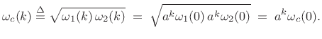 |
(12.121) |
Then
 |
(12.122) |
which does not depend on
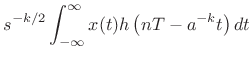
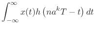
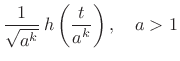
Discrete Wavelet Filterbank
In a discrete wavelet filterbank, each basis signal is
interpreted as the impulse response of a bandpass filter in a
constant-Q filter bank:
 |
|||
Thus, the
Recall that in the STFT, channel filter
![]() is a shift of
the zeroth channel-filter
is a shift of
the zeroth channel-filter
![]() (which corresponds to ``cosine
modulation'' in the time domain).
(which corresponds to ``cosine
modulation'' in the time domain).
As the channel-number ![]() increases, the channel impulse response
increases, the channel impulse response
![]() lengthens by the factor
lengthens by the factor ![]() ., while the pass-band of its
frequency-response
., while the pass-band of its
frequency-response ![]() narrows by the inverse factor
narrows by the inverse factor ![]() .
.
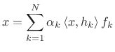
Figure 11.32 shows a block diagram of the discrete wavelet
filter bank for ![]() (the ``dyadic'' or ``octave filter-bank'' case),
and Fig.11.33 shows its time-frequency tiling as compared to
that of the STFT. The synthesis filters
(the ``dyadic'' or ``octave filter-bank'' case),
and Fig.11.33 shows its time-frequency tiling as compared to
that of the STFT. The synthesis filters ![]() may be used to make
a biorthogonal filter bank. If the
may be used to make
a biorthogonal filter bank. If the ![]() are orthonormal, then
are orthonormal, then
![]() .
.
![\includegraphics[width=\twidth]{eps/DyadicFilterbank}](http://www.dsprelated.com/josimages_new/sasp2/img2371.png)
![\includegraphics[width=0.8\twidth]{eps/DyadicTiling}](http://www.dsprelated.com/josimages_new/sasp2/img2372.png) |
Dyadic Filter Banks
![\includegraphics[width=0.7\twidth]{eps/dyadicFilters}](http://www.dsprelated.com/josimages_new/sasp2/img2373.png)
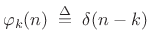
A dyadic filter bank is any octave filter
bank,12.6 as illustrated qualitatively in Figure 11.34. Note that
![]() is the top-octave bandpass filter,
is the top-octave bandpass filter,
![]() is the bandpass filter for next octave down,
is the bandpass filter for next octave down,
![]() is the octave bandpass below that, and so on. The optional
scale factors result in the same sum-of-squares for each
channel-filter impulse response.
is the octave bandpass below that, and so on. The optional
scale factors result in the same sum-of-squares for each
channel-filter impulse response.
A dyadic filter bank may be derived from the discrete wavelet filter
bank by setting ![]() and relaxing the exact orthonormality
requirement on the channel-filter impulse responses. If they do
happen to be orthonormal, we may call it a dyadic wavelet filter
bank.
and relaxing the exact orthonormality
requirement on the channel-filter impulse responses. If they do
happen to be orthonormal, we may call it a dyadic wavelet filter
bank.
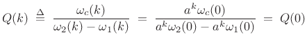
For a dyadic filter bank, the center-frequency of the ![]() th
channel-filter impulse response can be defined as
th
channel-filter impulse response can be defined as
| (12.123) |
so that
 |
(12.124) |
Thus, a dyadic filter bank is a special case of a constant-Q filter bank for which the
Dyadic Filter Bank Design
Design of dyadic filter banks using the window method for FIR digital filter design (introduced in §4.5) is described in, e.g., [226, §6.2.3b].
A ``very easy'' method suggested in [287, §11.6] is to design a two-channel paraunitary QMF bank, and repeat recursively to split the lower-half of the spectrum down to some desired depth.
Generalized STFT
A generalized STFT may be defined by [287]
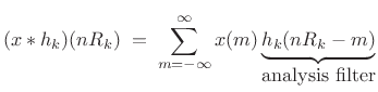 |
|||
 |
This filter bank and its reconstruction are diagrammed in Fig.11.35.
![\includegraphics[width=\twidth]{eps/GenSTFT}](http://www.dsprelated.com/josimages_new/sasp2/img2383.png)
The analysis filter ![]() is typically complex bandpass (as in the
STFT case). The integers
is typically complex bandpass (as in the
STFT case). The integers ![]() give the downsampling factor for the
output of the
give the downsampling factor for the
output of the ![]() th channel filter: For critical sampling without
aliasing, we set
th channel filter: For critical sampling without
aliasing, we set
![]() . The impulse response of
synthesis filter
. The impulse response of
synthesis filter ![]() can be regarded as the
can be regarded as the ![]() th basis
signal in the reconstruction. If the
th basis
signal in the reconstruction. If the ![]() are orthonormal, then
we have
are orthonormal, then
we have
![]() . More generally,
. More generally,
![]() form
a biorthogonal basis.
form
a biorthogonal basis.
Next Section:
Duration and Bandwidth as Second Moments
Previous Section:
Sliding FFT (Maximum Overlap), Any Window, Zero-Padded by 5


