


Getting Closer to Maximum Likelihood
In applications for which the fundamental frequency ![]() must be
measured very accurately in a periodic signal, the estimate obtained
by the above algorithm can be refined using a gradient search
which matches a so-called harmonic comb to the magnitude
spectrum of an interpolated FFT
must be
measured very accurately in a periodic signal, the estimate obtained
by the above algorithm can be refined using a gradient search
which matches a so-called harmonic comb to the magnitude
spectrum of an interpolated FFT ![]() :
:
![$\displaystyle \arg\max_{{\hat f}_0} \sum_{k=1}^K
\log\left[\left\vert X(k{\hat f}_0)\right\vert+\epsilon\right]$](http://www.dsprelated.com/josimages_new/sasp2/img1721.png)
![$\displaystyle \arg\max_{{\hat f}_0} \prod_{k=1}^K \left[\left\vert X(k{\hat f}_0)\right\vert+\epsilon\right]
\protect$](http://www.dsprelated.com/josimages_new/sasp2/img1722.png)
where
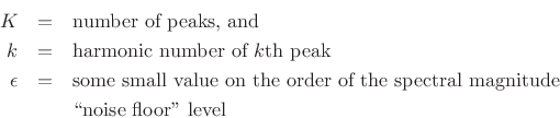
The purpose of
![]() is an insurance against multiplying the
whole expression by zero due to a missing partial (e.g., due to a
comb-filtering null). If
is an insurance against multiplying the
whole expression by zero due to a missing partial (e.g., due to a
comb-filtering null). If
![]() in (10.1), it is
advisable to omit indices
in (10.1), it is
advisable to omit indices ![]() for which
for which
![]() is too close to a
spectral null, since even one spectral null can push the product of
peak amplitudes to a very small value. At the same time, the product
should be penalized in some way to reflect the fact that it has fewer
terms (
is too close to a
spectral null, since even one spectral null can push the product of
peak amplitudes to a very small value. At the same time, the product
should be penalized in some way to reflect the fact that it has fewer
terms (
![]() is one way to accomplish this).
is one way to accomplish this).
As a practical matter, it is important to inspect the magnitude
spectra of the data frame manually to ensure that a robust row of
peaks is being matched by the harmonic comb. For example, it is
typical to look at a display of the frame magnitude spectrum overlaid
with vertical lines at the optimized harmonic-comb frequencies. This
provides an effective picture of the ![]() estimate in which typical
problems (such as octave errors) are readily seen.
estimate in which typical
problems (such as octave errors) are readily seen.
Next Section:
References on Estimation
Previous Section:
Useful Preprocessing


