


Linear Prediction Spectral Envelope
Linear Prediction (LP) implicitly computes a spectral envelope that is well adapted for audio work, provided the order of the predictor is appropriately chosen. Due to the error minimized by LP, spectral peaks are emphasized in the envelope, as they are in the auditory system. (The peak-emphasis of LP is quantified in (10.10) below.)
The term ``linear prediction'' refers to the process of predicting a
signal sample ![]() based on
based on ![]() past samples:
past samples:
We call
Taking the z transform of (10.4) yields
 |
(11.5) |
where
 |
(11.6) |
where
 |
(11.7) |
over some range of
If the prediction-error is successfully whitened, then the signal model can be expressed in the frequency domain as
 |
(11.8) |
where
| EnvelopeLPC |
(11.9) |
Linear Prediction is Peak Sensitive
By Rayleigh's energy theorem,
![]() (as
shown in §2.3.8). Therefore,
(as
shown in §2.3.8). Therefore,

From this ``ratio error'' expression in the frequency domain, we can see that contributions to the error are smallest when
Linear Prediction Methods
The two classic methods for linear prediction are called the autocorrelation method and the covariance method [162,157]. Both methods solve the linear normal equations (defined below) using different autocorrelation estimates.
In the autocorrelation method of linear prediction, the covariance
matrix is constructed from the usual Bartlett-window-biased sample
autocorrelation function (see Chapter 6), and it has the
desirable property that
![]() is always minimum phase (i.e.,
is always minimum phase (i.e.,
![]() is guaranteed to be stable). However, the autocorrelation
method tends to overestimate formant bandwidths; in other words, the
filter model is typically overdamped. This can be attributed to
implicitly ``predicting zero'' outside of the signal frame, resulting
in the Bartlett-window bias in the sample autocorrelation.
is guaranteed to be stable). However, the autocorrelation
method tends to overestimate formant bandwidths; in other words, the
filter model is typically overdamped. This can be attributed to
implicitly ``predicting zero'' outside of the signal frame, resulting
in the Bartlett-window bias in the sample autocorrelation.
The covariance method of LP is based on an unbiased
autocorrelation estimate (see Eq.![]() (6.4)). As a result, it
gives more accurate bandwidths, but it does not guarantee stability.
(6.4)). As a result, it
gives more accurate bandwidths, but it does not guarantee stability.
So-called covariance lattice methods and Burg's method were developed to maintain guaranteed stability while giving accuracy comparable to the covariance method of LP [157].
Computation of Linear Prediction Coefficients
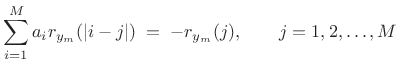
In the autocorrelation method of linear prediction, the linear
prediction coefficients
![]() are computed from the
Bartlett-window-biased autocorrelation function
(Chapter 6):
are computed from the
Bartlett-window-biased autocorrelation function
(Chapter 6):
where
In matlab syntax, the solution is given by ``
If the rank of the ![]() autocorrelation matrix
autocorrelation matrix
![]() is
is ![]() , then the solution to (10.12)
is unique, and
this solution is always minimum phase [162] (i.e., all roots of
, then the solution to (10.12)
is unique, and
this solution is always minimum phase [162] (i.e., all roots of
![]() are inside the unit circle in the
are inside the unit circle in the ![]() plane [263], so
that
plane [263], so
that ![]() is always a stable all-pole filter). In
practice, the rank of
is always a stable all-pole filter). In
practice, the rank of ![]() is
is ![]() (with probability 1) whenever
(with probability 1) whenever ![]() includes a noise component. In the noiseless case, if
includes a noise component. In the noiseless case, if ![]() is a sum
of sinusoids, each (real) sinusoid at distinct frequency
is a sum
of sinusoids, each (real) sinusoid at distinct frequency
![]() adds 2 to the rank. A dc component, or a component at half the
sampling rate, adds 1 to the rank of
adds 2 to the rank. A dc component, or a component at half the
sampling rate, adds 1 to the rank of ![]() .
.
The choice of time window for forming a short-time sample
autocorrelation and its weighting also affect the rank of
![]() . Equation (10.11) applied to a finite-duration frame yields what is
called the autocorrelation method of linear
prediction [162]. Dividing out the Bartlett-window bias in such a
sample autocorrelation yields a result closer to the covariance method
of LP. A matlab example is given in §10.3.3 below.
. Equation (10.11) applied to a finite-duration frame yields what is
called the autocorrelation method of linear
prediction [162]. Dividing out the Bartlett-window bias in such a
sample autocorrelation yields a result closer to the covariance method
of LP. A matlab example is given in §10.3.3 below.
The classic covariance method computes an unbiased sample covariance
matrix by limiting the summation in (10.11) to a range over which
![]() stays within the frame--a so-called ``unwindowed'' method.
The autocorrelation method sums over the whole frame and replaces
stays within the frame--a so-called ``unwindowed'' method.
The autocorrelation method sums over the whole frame and replaces
![]() by zero when
by zero when ![]() points outside the frame--a so-called
``windowed'' method (windowed by the rectangular window).
points outside the frame--a so-called
``windowed'' method (windowed by the rectangular window).
Linear Prediction Order Selection
For computing spectral envelopes via linear prediction, the order ![]() of the predictor should be chosen large enough that the envelope can
follow the contour of the spectrum, but not so large that it follows
the spectral ``fine structure'' on a scale not considered to belong in
the envelope. In particular, for voice,
of the predictor should be chosen large enough that the envelope can
follow the contour of the spectrum, but not so large that it follows
the spectral ``fine structure'' on a scale not considered to belong in
the envelope. In particular, for voice, ![]() should be twice the
number of spectral formants, and perhaps a little larger to
allow more detailed modeling of spectral shape away from the formants.
For a sum of quasi sinusoids, the order
should be twice the
number of spectral formants, and perhaps a little larger to
allow more detailed modeling of spectral shape away from the formants.
For a sum of quasi sinusoids, the order ![]() should be significantly
less than twice the number of sinusoids to inhibit modeling the
sinusoids as spectral-envelope peaks. For filtered-white-noise,
should be significantly
less than twice the number of sinusoids to inhibit modeling the
sinusoids as spectral-envelope peaks. For filtered-white-noise, ![]() should be close to the order of the filter applied to the white noise,
and so on.
should be close to the order of the filter applied to the white noise,
and so on.
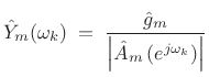
Summary of LP Spectral Envelopes
In summary, the spectral envelope of the ![]() th spectral frame,
computed by linear prediction, is given by
th spectral frame,
computed by linear prediction, is given by
 |
(11.13) |
where
 |
(11.14) |
can be driven by unit-variance white noise to produce a filtered-white-noise signal having spectral envelope
It bears repeating that
![]() is zero mean when
is zero mean when
![]() is monic and minimum phase (all zeros inside the unit circle).
This means, for example, that
is monic and minimum phase (all zeros inside the unit circle).
This means, for example, that
![]() can be simply estimated as
the mean of the log spectral magnitude
can be simply estimated as
the mean of the log spectral magnitude
![]() .
.
For best results, the frequency axis ``seen'' by linear prediction should be warped to an auditory frequency scale, as discussed in Appendix E [123]. This has the effect of increasing the accuracy of low-frequency peaks in the extracted spectral envelope, in accordance with the nonuniform frequency resolution of the inner ear.
Next Section:
Spectral Envelope Examples
Previous Section:
Cepstral Windowing


