


Maximum Entropy Property of the
Gaussian Distribution
Entropy of a Probability Distribution
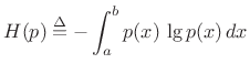
The entropy of a probability density function (PDF) ![]() is
defined as [48]
is
defined as [48]
![$\displaystyle \zbox {h(p) \isdef \int_x p(x) \cdot \lg\left[\frac{1}{p(x)}\right] dx}$](http://www.dsprelated.com/josimages_new/sasp2/img2794.png) |
(D.29) |
where
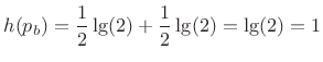
![$\displaystyle h(p) = {\cal E}_p\left\{\lg \left[\frac{1}{p(x)}\right]\right\}$](http://www.dsprelated.com/josimages_new/sasp2/img2796.png) |
(D.30) |
The term
Example: Random Bit String
Consider a random sequence of 1s and 0s, i.e., the probability of a 0 or
1 is always
![]() . The corresponding probability density function
is
. The corresponding probability density function
is
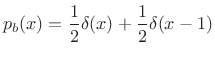 |
(D.31) |
and the entropy is
 |
(D.32) |
Thus, 1 bit is required for each bit of the sequence. In other words, the sequence cannot be compressed. There is no redundancy.
If instead the probability of a 0 is 1/4 and that of a 1 is 3/4, we get
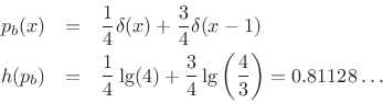
and the sequence can be compressed about ![]() .
.
In the degenerate case for which the probability of a 0 is 0 and that of a 1 is 1, we get
![\begin{eqnarray*}
p_b(x) &=& \lim_{\epsilon \to0}\left[\epsilon \delta(x) + (1-\epsilon )\delta(x-1)\right]\\
h(p_b) &=& \lim_{\epsilon \to0}\epsilon \cdot\lg\left(\frac{1}{\epsilon }\right) + 1\cdot\lg(1) = 0.
\end{eqnarray*}](http://www.dsprelated.com/josimages_new/sasp2/img2803.png)
Thus, the entropy is 0 when the sequence is perfectly predictable.
Maximum Entropy Distributions
Uniform Distribution
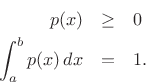
Among probability distributions ![]() which are nonzero over a
finite range of values
which are nonzero over a
finite range of values ![]() , the maximum-entropy
distribution is the uniform distribution. To show this, we
must maximize the entropy,
, the maximum-entropy
distribution is the uniform distribution. To show this, we
must maximize the entropy,
 |
(D.33) |
with respect to
Using the method of Lagrange multipliers for optimization in the presence of constraints [86], we may form the objective function
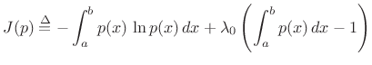 |
(D.34) |
and differentiate with respect to
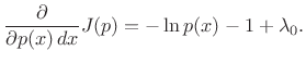 |
(D.35) |
Setting this to zero and solving for
| (D.36) |
(Setting the partial derivative with respect to
Choosing ![]() to satisfy the constraint gives
to satisfy the constraint gives
![]() , yielding
, yielding
![$\displaystyle p(x) = \left\{\begin{array}{ll} \frac{1}{b-a}, & a\leq x \leq b \\ [5pt] 0, & \hbox{otherwise}. \\ \end{array} \right.$](http://www.dsprelated.com/josimages_new/sasp2/img2812.png) |
(D.37) |
That this solution is a maximum rather than a minimum or inflection point can be verified by ensuring the sign of the second partial derivative is negative for all
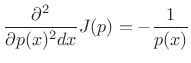 |
(D.38) |
Since the solution spontaneously satisfied
Exponential Distribution
Among probability distributions ![]() which are nonzero over a
semi-infinite range of values
which are nonzero over a
semi-infinite range of values
![]() and having a finite
mean
and having a finite
mean ![]() , the exponential distribution has maximum entropy.
, the exponential distribution has maximum entropy.
To the previous case, we add the new constraint
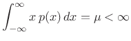 |
(D.39) |
resulting in the objective function
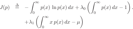
Now the partials with respect to ![]() are
are
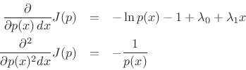
and ![]() is of the form
is of the form
![]() . The
unit-area and finite-mean constraints result in
. The
unit-area and finite-mean constraints result in
![]() and
and
![]() , yielding
, yielding
![$\displaystyle p(x) = \left\{\begin{array}{ll} \frac{1}{\mu} e^{-x/\mu}, & x\geq 0 \\ [5pt] 0, & \hbox{otherwise}. \\ \end{array} \right.$](http://www.dsprelated.com/josimages_new/sasp2/img2822.png) |
(D.40) |
Gaussian Distribution
The Gaussian distribution has maximum entropy relative to all
probability distributions covering the entire real line
![]() but having a finite mean
but having a finite mean ![]() and finite
variance
and finite
variance ![]() .
.
Proceeding as before, we obtain the objective function
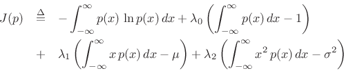
and partial derivatives
leading to
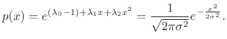 |
(D.41) |
For more on entropy and maximum-entropy distributions, see [48].
Next Section:
Gaussian Moments
Previous Section:
Gaussian Probability Density Function


