


Maximum Likelihood Sinusoid Estimation
The maximum likelihood estimator (MLE) is widely used in practical signal modeling [121]. A full treatment of maximum likelihood estimators (and statistical estimators in general) lies beyond the scope of this book. However, we will show that the MLE is equivalent to the least squares estimator for a wide class of problems, including well resolved sinusoids in white noise.
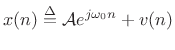
Consider again the signal model of (5.32) consisting of a complex sinusoid in additive white (complex) noise:
Again,
 |
(6.46) |
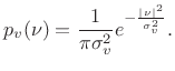
We express the zero-mean Gaussian assumption by writing
| (6.47) |
The parameter
It turns out that when Gaussian random variables ![]() are
uncorrelated (i.e., when
are
uncorrelated (i.e., when ![]() is white noise), they are also
independent. This means that the probability of observing
particular values of
is white noise), they are also
independent. This means that the probability of observing
particular values of ![]() and
and ![]() is given by the product of
their respective probabilities [121]. We will now use this
fact to compute an explicit probability for observing any data
sequence
is given by the product of
their respective probabilities [121]. We will now use this
fact to compute an explicit probability for observing any data
sequence ![]() in (5.44).
in (5.44).
Since the sinusoidal part of our signal model,
![]() , is deterministic; i.e., it does not including any random
components; it may be treated as the time-varying mean of a
Gaussian random process
, is deterministic; i.e., it does not including any random
components; it may be treated as the time-varying mean of a
Gaussian random process ![]() . That is, our signal model
(5.44) can be rewritten as
. That is, our signal model
(5.44) can be rewritten as
| (6.48) |
and the probability density function for the whole set of observations
![$\displaystyle p(x) = p[x(0)] p[x(1)]\cdots p[x(N-1)] = \left(\frac{1}{\pi \sigma_v^2}\right)^N e^{-\frac{1}{\sigma_v^2}\sum_{n=0}^{N-1} \left\vert x(n) - {\cal A}e^{j\omega_0 n}\right\vert^2}$](http://www.dsprelated.com/josimages_new/sasp2/img1079.png) |
(6.49) |
Thus, given the noise variance
Next Section:
Likelihood Function
Previous Section:
Least Squares Sinusoidal Parameter Estimation


