


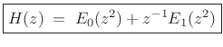
Multirate Filter Banks
The preceding chapters have been concerned essentially with the short-time Fourier transform and all that goes with it. After developing the overlap-add point of view in Chapter 8, we developed the alternative (dual) filter-bank point of view in Chapter 9. This chapter is concerned more broadly with filter banks, whether they are implemented using an FFT or by some other means. In the end, however, we will come full circle and look at the properly configured STFT as an example of a perfect reconstruction (PR) filter bank as defined herein. Moreover, filter banks in practice are normally implemented using FFT methods.
The subject of PR filter banks is normally considered only in the context of systems for audio compression, and they are normally critically sampled in both time and frequency. This book, on the other hand, belongs to a tiny minority which is not concerned with compression at all, but rather useful time-frequency decompositions for sound, and corresponding applications in music and digital audio effects.
Perhaps the most important new topic introduced in this chapter is the polyphase representation for filter banks. This is both an important analysis tool and a basis for efficient implementation. We will see that it can be seen as a generalization of the overlap-add approach discussed in Chapter 8.
The polyphase representation will make it straightforward to determine general conditions for perfect reconstruction in any filter bank. The STFT will provide some special cases, but there will be many more. In particular, the filter banks used in perceptual audio coding will be special cases as well. Polyphase analysis is used to derive classes of PR filter banks called ``paraunitary,'' ``cosine modulated,'' and ``pseudo-quadrature mirror'' filter banks, among others.
Another extension we will take up in this chapter is multirate systems. Multirate filter banks use different sampling rates in different channels, matched to different filter bandwidths. Multirate filter banks are very important in audio work because the filtering by the inner ear is similarly a variable resolution ``filter bank'' using wider pass-bands at higher frequencies. Finally, the related subject of wavelet filter banks is briefly introduced, and further reading is recommended.
Upsampling and Downsampling
For the DTFT, we proved in Chapter 2 (p.
p. ![]() ) the stretch theorem (repeat theorem) which
relates upsampling (``stretch'') to spectral copies (``images'') in
the DTFT context; this is the discrete-time counterpart of the scaling
theorem for continuous-time Fourier transforms
(§B.4). Also, §2.3.12 discusses the downsampling
theorem (aliasing theorem) for DTFTs which relates downsampling to
aliasing for discrete-time signals. In this section, we review the
main results.
) the stretch theorem (repeat theorem) which
relates upsampling (``stretch'') to spectral copies (``images'') in
the DTFT context; this is the discrete-time counterpart of the scaling
theorem for continuous-time Fourier transforms
(§B.4). Also, §2.3.12 discusses the downsampling
theorem (aliasing theorem) for DTFTs which relates downsampling to
aliasing for discrete-time signals. In this section, we review the
main results.
Upsampling (Stretch) Operator
Figure 11.1 shows the graphical symbol for a digital upsampler
by the factor ![]() . To upsample by the integer factor
. To upsample by the integer factor ![]() , we simply
insert
, we simply
insert ![]() zeros between
zeros between ![]() and
and ![]() for all
for all ![]() . In other
words, the upsampler implements the stretch operator defined
in §2.3.9:
. In other
words, the upsampler implements the stretch operator defined
in §2.3.9:
![\begin{eqnarray*}
y(n) &=& \hbox{\sc Stretch}_{N,n}(x)\\
&\isdef & \left\{\begin{array}{ll}
x(n/N), & \frac{n}{N}\in{\bf Z} \\ [5pt]
0, & \hbox{otherwise}. \\
\end{array} \right.
\end{eqnarray*}](http://www.dsprelated.com/josimages_new/sasp2/img1924.png)
In the frequency domain, we have, by the stretch (repeat) theorem for DTFTs:
Plugging in
![]() , we see that the spectrum on
, we see that the spectrum on
![]() contracts by the factor
contracts by the factor ![]() , and
, and ![]() images appear around the
unit circle. For
images appear around the
unit circle. For ![]() , this is depicted in Fig.11.2.
, this is depicted in Fig.11.2.
![\includegraphics[width=0.8\twidth]{eps/upsampspec}](http://www.dsprelated.com/josimages_new/sasp2/img1927.png)
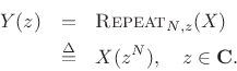
Downsampling (Decimation) Operator
Figure 11.3 shows the symbol for downsampling by the factor ![]() .
The downsampler selects every
.
The downsampler selects every ![]() th sample and discards the rest:
th sample and discards the rest:

In the frequency domain, we have
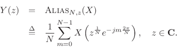
Thus, the frequency axis is expanded by the factor ![]() , wrapping
, wrapping
![]() times around the unit circle, adding to itself
times around the unit circle, adding to itself ![]() times. For
times. For
![]() , two partial spectra are summed, as indicated in Fig.11.4.
, two partial spectra are summed, as indicated in Fig.11.4.
![\includegraphics[width=0.8\twidth]{eps/dnsampspec}](http://www.dsprelated.com/josimages_new/sasp2/img1931.png)
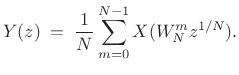
Using the common twiddle factor notation
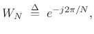 |
(12.1) |
the aliasing expression can be written as
Example: Downsampling by 2
For ![]() , downsampling by 2 can be expressed as
, downsampling by 2 can be expressed as
![]() , so that
(since
, so that
(since
 )
)
![\begin{eqnarray*}
Y(z) &=& \frac{1}{2}\left[X\left(W^0_2 z^{1/2}\right) + X\left(W^1_2 z^{1/2}\right)\right] \\ [5pt]
&=& \frac{1}{2}\left[X\left(e^{-j2\pi 0/2} z^{1/2}\right) + X\left(e^{-j2\pi 1/2}z^{1/2}\right)\right] \\ [5pt]
&=& \frac{1}{2}\left[X\left(z^{1/2}\right) + X\left(-z^{1/2}\right)\right] \\ [5pt]
&=& \frac{1}{2}\left[\hbox{\sc Stretch}_2(X) + \hbox{\sc Stretch}_2\left(\hbox{\sc Shift}_\pi(X)\right)\right].
\end{eqnarray*}](http://www.dsprelated.com/josimages_new/sasp2/img1936.png)
Example: Upsampling by 2
For ![]() , upsampling (stretching) by 2 can be expressed as
, upsampling (stretching) by 2 can be expressed as
![]() , so that
, so that
| (12.2) |
as discussed more fully in §2.3.11.
Filtering and Downsampling
Because downsampling by ![]() causes aliasing of any frequencies in the
original signal above
causes aliasing of any frequencies in the
original signal above
![]() , the input signal may need to
be first lowpass-filtered to prevent this aliasing, as shown in
Fig.11.5.
, the input signal may need to
be first lowpass-filtered to prevent this aliasing, as shown in
Fig.11.5.
Suppose we implement such an anti-aliasing lowpass filter ![]() as an
FIR filter of length
as an
FIR filter of length ![]() with cut-off frequency
with cut-off frequency
![]() .12.1 This is drawn in direct form in
Fig.11.6.
.12.1 This is drawn in direct form in
Fig.11.6.
![\includegraphics[width=0.6\twidth]{eps/down_FIR}](http://www.dsprelated.com/josimages_new/sasp2/img1943.png) |
![\includegraphics[width=0.6\twidth]{eps/down_FIR_com}](http://www.dsprelated.com/josimages_new/sasp2/img1944.png)
We do not need ![]() out of every
out of every ![]() filter output samples due to the
filter output samples due to the
![]() :
:![]() downsampler. To realize this savings, we can commute the
downsampler through the adders inside the FIR filter to obtain the
result shown in Fig.11.7. The multipliers are now running
at
downsampler. To realize this savings, we can commute the
downsampler through the adders inside the FIR filter to obtain the
result shown in Fig.11.7. The multipliers are now running
at ![]() times the sampling frequency of the input signal
times the sampling frequency of the input signal ![]() .
This reduces the computation requirements by a factor of
.
This reduces the computation requirements by a factor of ![]() . The
downsampler outputs in Fig.11.7 are called polyphase
signals. The overall system is a summed polyphase filter
bank in which each ``subphase filter'' is a constant scale factor
. The
downsampler outputs in Fig.11.7 are called polyphase
signals. The overall system is a summed polyphase filter
bank in which each ``subphase filter'' is a constant scale factor
![]() . As we will see, more general subphase filters can be used to
implement time-domain aliasing as needed for Portnoff windows
(§9.7).
. As we will see, more general subphase filters can be used to
implement time-domain aliasing as needed for Portnoff windows
(§9.7).
We may describe the polyphase processing in the anti-aliasing filter of Fig.11.7 as follows:
- Subphase signal 0
![$\displaystyle x(nN)\left\vert _{n=0}^{\infty}\right. \eqsp [x_0,x_N,x_{2N},\ldots]$](http://www.dsprelated.com/josimages_new/sasp2/img1947.png)
(12.3)
is scaled by .
.
- Subphase signal 1
![$\displaystyle x(nN-1)\left\vert _{n=0}^{\infty}\right.\eqsp [x_{-1},x_{N-1},x_{2N-1},\ldots]$](http://www.dsprelated.com/josimages_new/sasp2/img1948.png)
(12.4)
is scaled by ,
,

- Subphase signal

![$\displaystyle x(nN-m)\left\vert _{n=0}^{\infty}\right.\eqsp [x_{-m},x_{N-m},x_{2N-m},\ldots]
$](http://www.dsprelated.com/josimages_new/sasp2/img1951.png)
is scaled by .
.
 |
(12.5) |
which we recognize as a direct-form-convolution implementation of a length
The summed polyphase signals of Fig.11.7 can be interpreted
as ``serial to parallel conversion'' from an ``interleaved'' stream of
scalar samples ![]() to a ``deinterleaved'' sequence of buffers (each
length
to a ``deinterleaved'' sequence of buffers (each
length ![]() ) every
) every ![]() samples, followed by an inner product of each
buffer with
samples, followed by an inner product of each
buffer with
![]() . The same operation may be
visualized as a deinterleaving through variable gains into a running
sum, as shown in Fig.11.8.
. The same operation may be
visualized as a deinterleaving through variable gains into a running
sum, as shown in Fig.11.8.
![\includegraphics[width=0.7\twidth]{eps/periodicGain}](http://www.dsprelated.com/josimages_new/sasp2/img1955.png)
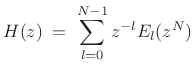
Polyphase Decomposition
The previous section derived an efficient polyphase implementation of
an FIR filter ![]() whose output was downsampled by the factor
whose output was downsampled by the factor ![]() . The
derivation was based on commuting the downsampler with the FIR
summer. We now derive the polyphase representation of a filter of any
length algebraically by splitting the impulse response
. The
derivation was based on commuting the downsampler with the FIR
summer. We now derive the polyphase representation of a filter of any
length algebraically by splitting the impulse response ![]() into
into
![]() polyphase components.
polyphase components.
Two-Channel Case
The simplest nontrivial case is ![]() channels. Starting with a
general linear time-invariant filter
channels. Starting with a
general linear time-invariant filter
 |
(12.6) |
we may separate the even- and odd-indexed terms to get
 |
(12.7) |
We define the polyphase component filters as follows:
![\begin{eqnarray*}
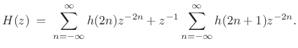
E_0(z)&=&\sum_{n=-\infty}^{\infty}h(2n)z^{-n}\\ [5pt]
E_1(z)&=&\sum_{n=-\infty}^{\infty}h(2n+1)z^{-n}
\end{eqnarray*}](http://www.dsprelated.com/josimages_new/sasp2/img1958.png)
![]() and
and ![]() are the polyphase components
of the polyphase decomposition of
are the polyphase components
of the polyphase decomposition of ![]() for
for ![]() .
.
Now write ![]() in terms of its polyphase components:
in terms of its polyphase components:
 |
(12.8) |
As a simple example, consider
| (12.9) |
Then the polyphase component filters are
![\begin{eqnarray*}
E_0(z) &=& 1 + 3z^{-1}\\ [5pt]
E_1(z) &=& 2 + 4z^{-1}
\end{eqnarray*}](http://www.dsprelated.com/josimages_new/sasp2/img1963.png)
and
| (12.10) |
N-Channel Polyphase Decomposition
![\includegraphics[scale=0.8]{eps/polytime}](http://www.dsprelated.com/josimages_new/sasp2/img1965.png)
For the general case of arbitrary ![]() , the basic idea is to decompose
, the basic idea is to decompose
![]() into its periodically interleaved subsequences, as indicated
schematically in Fig.11.9. The polyphase decomposition into
into its periodically interleaved subsequences, as indicated
schematically in Fig.11.9. The polyphase decomposition into
![]() channels is given by
channels is given by
where the subphase filters are defined by
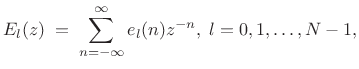 |
(12.12) |
with
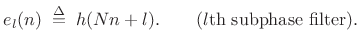 |
(12.13) |
The signal
![\begin{psfrags}
% latex2html id marker 29755\psfrag{M}{{\normalsize $N$}}\psfrag{ztl}{{\Large $z^l$}}\psfrag{h[n]}{{\Large $h(n)$}}\psfrag{eln}{{\Large $e_l(n)$}}\begin{figure}[htbp]
\includegraphics[width=0.5\twidth]{eps/polypick}
\caption{Advance by $l$\ samples followed by a downsampling by the factor $N$.}
\end{figure}
\end{psfrags}](http://www.dsprelated.com/josimages_new/sasp2/img1970.png)
Type II Polyphase Decomposition
The polyphase decomposition of ![]() into
into ![]() channels in
(11.11) may be termed a ``type I'' polyphase decomposition. In
the ``type II'', or reverse polyphase decomposition, the powers
of
channels in
(11.11) may be termed a ``type I'' polyphase decomposition. In
the ``type II'', or reverse polyphase decomposition, the powers
of ![]() progress in the opposite direction:
progress in the opposite direction:
 |
(12.14) |
We will see that we need type I for analysis filter banks and type II for synthesis filter banks in a general ``perfect reconstruction filter bank'' analysis/synthesis system.
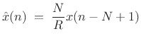
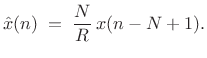
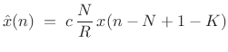
Filtering and Downsampling, Revisited
Let's return to the example of §11.1.3, but
this time have the FIR lowpass filter h(n) be length ![]() ,
,
![]() . In this case, the
. In this case, the ![]() polyphase filters,
polyphase filters, ![]() , are
each length
, are
each length ![]() .12.2 Recall that
.12.2 Recall that
| (12.15) |
leading to the result shown in Fig.11.11.
![\includegraphics[width=0.7\twidth]{eps/down_FIR_poly}](http://www.dsprelated.com/josimages_new/sasp2/img1974.png)
![\includegraphics[width=0.7\twidth]{eps/down_FIR_poly_com}](http://www.dsprelated.com/josimages_new/sasp2/img1975.png)
Next, we commute the ![]() :
:![]() downsampler through the adders and
upsampled (stretched) polyphase filters
downsampler through the adders and
upsampled (stretched) polyphase filters ![]() to obtain
Fig.11.12. Commuting the downsampler through the
subphase filters
to obtain
Fig.11.12. Commuting the downsampler through the
subphase filters ![]() to obtain
to obtain ![]() is an example of a
multirate noble identity.
is an example of a
multirate noble identity.
Multirate Noble Identities
Figure 11.13 illustrates the so-called noble identities for
commuting downsamplers/upsamplers with ``sparse transfer functions''
that can be expressed a function of ![]() . Note that downsamplers
and upsamplers are linear, time-varying operators. Therefore,
operation order is important. Also note that adders and multipliers
(any memoryless operators) may be commuted across downsamplers and
upsamplers, as shown in Fig.11.14.
. Note that downsamplers
and upsamplers are linear, time-varying operators. Therefore,
operation order is important. Also note that adders and multipliers
(any memoryless operators) may be commuted across downsamplers and
upsamplers, as shown in Fig.11.14.
![\begin{psfrags}
% latex2html id marker 29805\psfrag{nd}{ $N\downarrow$\ }\psfrag{hz}{ $H(z)$\ }\psfrag{hzn}{ $H(z^N)$\ }\psfrag{equal}{ $\equiv$\ }\begin{figure}[htbp]
\includegraphics[width=0.9\twidth]{eps/noble}
\caption{Multirate noble identities}
\end{figure} % was 6in
\end{psfrags}](http://www.dsprelated.com/josimages_new/sasp2/img1979.png)
![\includegraphics[width=0.9\twidth]{eps/noble_commute}](http://www.dsprelated.com/josimages_new/sasp2/img1980.png)
Critically Sampled Perfect Reconstruction Filter Banks
A Perfect Reconstruction (PR) filter bank is any filter bank
whose reconstruction is the original signal, possibly delayed, and
possibly scaled by a constant [287]. In this context,
critical sampling (also called ``maximal downsampling'') means
that the downsampling factor is the same as the number of filter
channels. For the STFT, this implies ![]() (with
(with ![]() allowed for
Portnoff windows).
allowed for
Portnoff windows).
As derived in Chapter 8, the Short-Time Fourier
Transform (STFT) is a PR filter bank whenever the Constant-OverLap-Add
(COLA) condition is met by the analysis window ![]() and the hop size
and the hop size
![]() . However, only the rectangular window case with no
zero-padding is critically sampled (OLA hop size = FBS downsampling
factor =
. However, only the rectangular window case with no
zero-padding is critically sampled (OLA hop size = FBS downsampling
factor = ![]() ). Perceptual audio compression algorithms such as MPEG
audio coding are based on critically sampled filter banks, for obvious
reasons. It is important to remember that we normally do not require
critical sampling for audio analysis, digital audio effects, and music
applications; instead, we normally need critical sampling only when
compression is a requirement. Thus, when compression is not a
requirement, we are normally interested in oversampled filter
banks. The polyphase representation is useful in that case as
well. In particular, we will obtain some excellent insights into the
aliasing cancellation that goes on in such downsampled filter
banks (including STFTs with hop sizes
). Perceptual audio compression algorithms such as MPEG
audio coding are based on critically sampled filter banks, for obvious
reasons. It is important to remember that we normally do not require
critical sampling for audio analysis, digital audio effects, and music
applications; instead, we normally need critical sampling only when
compression is a requirement. Thus, when compression is not a
requirement, we are normally interested in oversampled filter
banks. The polyphase representation is useful in that case as
well. In particular, we will obtain some excellent insights into the
aliasing cancellation that goes on in such downsampled filter
banks (including STFTs with hop sizes ![]() ), as the next section
makes clear.
), as the next section
makes clear.
Two-Channel Critically Sampled Filter Banks
Figure 11.15 shows a simple two-channel band-splitting filter bank,
followed by the corresponding synthesis filter bank which
reconstructs the original signal (we hope) from the two channels. The
analysis filter ![]() is a half-band lowpass filter, and
is a half-band lowpass filter, and ![]() is a complementary half-band highpass filter. The synthesis filters
is a complementary half-band highpass filter. The synthesis filters
![]() and
and ![]() are to be derived. Intuitively, we expect
are to be derived. Intuitively, we expect
![]() to be a lowpass that rejects the upper half-band due to the
upsampler by 2, and
to be a lowpass that rejects the upper half-band due to the
upsampler by 2, and ![]() should do the same but then also
reposition its output band as the upper half-band, which can be
accomplished by selecting the upper of the two spectral images in the
upsampler output.
should do the same but then also
reposition its output band as the upper half-band, which can be
accomplished by selecting the upper of the two spectral images in the
upsampler output.
![\begin{psfrags}
% latex2html id marker 29839\psfrag{x(n)}{\normalsize $x(n)$}\psfrag{x}{\normalsize $x$}\psfrag{(n)}{\normalsize $(n)$}\psfrag{y}{\normalsize $y$}\psfrag{v}{\normalsize $v$}\psfrag{H}{\normalsize $H$}\psfrag{F}{\normalsize $F$}\psfrag{z}{\normalsize $z$}\begin{figure}[htbp]
\includegraphics[width=\twidth]{eps/cqf}
\caption{Two-channel critically sampled filter bank.}
\end{figure}
\end{psfrags}](http://www.dsprelated.com/josimages_new/sasp2/img1986.png)
The outputs of the two analysis filters in Fig.11.15 are
| (12.16) |
Using the results of §11.1, the signals become, after downsampling,
![$\displaystyle V_k(z) \eqsp \frac{1}{2}\left[X_k(z^{1/2}) + X_k(-z^{1/2})\right], \; k=0,1.$](http://www.dsprelated.com/josimages_new/sasp2/img1988.png) |
(12.17) |
After upsampling, the signals become
![$\displaystyle \frac{1}{2}[X_k(z) + X_k(-z)]$](http://www.dsprelated.com/josimages_new/sasp2/img1990.png) |
|||
![$\displaystyle \frac{1}{2}[H_k(z)X(z) + H_k(-z)X(-z)],\; k=0,1.$](http://www.dsprelated.com/josimages_new/sasp2/img1991.png) |
After substitutions and rearranging, we find that the output
![$\displaystyle \frac{1}{2}\left[H_0(z)F_0(z) + H_1(z)F_1(z)\right]X(z)$](http://www.dsprelated.com/josimages_new/sasp2/img1994.png)
![$\displaystyle \frac{1}{2}\left[H_0(-z)F_0(z) + H_1(-z)F_1(z)\right]X(-z)
\protect$](http://www.dsprelated.com/josimages_new/sasp2/img1996.png)
For perfect reconstruction, we require the aliasing term to be zero. For ideal half-band filters cutting off at
In this case, synthesis filter
Referring again to (11.18), we see that we also need the
non-aliased term to be of the form
where
| (12.21) |
That is, for perfect reconstruction, we need, in addition to aliasing cancellation, that the non-aliasing term reduce to a constant gain
Let
![]() denote
denote ![]() . Then both constraints can be expressed in
matrix form as follows:
. Then both constraints can be expressed in
matrix form as follows:
![$\displaystyle \left[\begin{array}{cc} H_0 & H_1 \\ [2pt] {\tilde H}_0 & {\tilde H}_1 \end{array}\right]\left[\begin{array}{c} F_0 \\ [2pt] F_1 \end{array}\right]\eqsp \left[\begin{array}{c} c \\ [2pt] 0 \end{array}\right]$](http://www.dsprelated.com/josimages_new/sasp2/img2013.png) |
(12.22) |
Substituting the aliasing-canceling choices for ![]() and
and ![]() from
(11.19) into the filtering-cancellation constraint (11.20), we
obtain
from
(11.19) into the filtering-cancellation constraint (11.20), we
obtain
The filtering-cancellation constraint is almost satisfied by ideal zero-phase half-band filters cutting off at
Amplitude-Complementary 2-Channel Filter Bank
A natural choice of analysis filters for our two-channel critically sampled filter bank is an amplitude-complementary lowpass/highpass pair, i.e.,
| (12.24) |
where we impose the unity dc gain constraint
Substituting the COLA constraint into the filtering and aliasing cancellation constraint (11.23) gives
![\begin{eqnarray*}
g\,z^{-d} &=& H_0(z)\left[1-H_0(-z)\right] - \left[1-H_0(z)\right]H_0(-z) \\ [5pt]
&=& H_0(z) - H_0(-z)\\ [5pt]
\;\longleftrightarrow\;\quad a(n) &=& h_0(n) - (-1)^n h_0(n) \\ [5pt]
&=& \left\{\begin{array}{ll}
0, & \hbox{$n$\ even} \\ [5pt]
2h_0(n), & \hbox{$n$\ odd} \\
\end{array} \right.
\end{eqnarray*}](http://www.dsprelated.com/josimages_new/sasp2/img2021.png)
Thus, we find that even-indexed terms of the impulse response are
unconstrained, since they subtract out in the constraint, while,
for perfect reconstruction, exactly one odd-indexed term
must be nonzero in the lowpass impulse response ![]() . The
simplest choice is
. The
simplest choice is
![]() .
.
Thus, we have derived that the lowpass-filter impulse-response for channel 0 can be anything of the form
or
| (12.26) |
etc. The corresponding highpass-filter impulse response is then
| (12.27) |
The first example (11.25) above goes with the highpass filter
| (12.28) |
and similarly for the other example.
The above class of amplitude-complementary filters can be characterized in general as follows:
![\begin{eqnarray*}
H_0(z) &=& E_0(z^2) + h_0(o) z^{-o}, \quad E_0(1)+h_0(o)\eqsp 1, \, \hbox{$o$\ odd}\\ [5pt]
H_1(z) &=& 1-H_0(z) \eqsp 1 - E_0(z^2) - h_0(o) z^{-o}
\end{eqnarray*}](http://www.dsprelated.com/josimages_new/sasp2/img2028.png)
In summary, we see that an amplitude-complementary
lowpass/highpass analysis filter pair yields perfect reconstruction
(aliasing and filtering cancellation) when there is exactly one
odd-indexed term in the impulse response of ![]() .
.
Unfortunately, the channel filters are so constrained in form that it
is impossible to make a high quality lowpass/highpass pair. This
happens because ![]() repeats twice around the unit circle. Since
we assume real coefficients, the frequency response,
repeats twice around the unit circle. Since
we assume real coefficients, the frequency response,
![]() is magnitude-symmetric about
is magnitude-symmetric about
![]() as
well as
as
well as ![]() . This is not good since we only have one degree of
freedom,
. This is not good since we only have one degree of
freedom,
![]() , with which we can break the
, with which we can break the ![]() symmetry
to reduce the high-frequency gain and/or boost the low-frequency gain.
This class of filters cannot be expected to give high quality lowpass
or highpass behavior.
symmetry
to reduce the high-frequency gain and/or boost the low-frequency gain.
This class of filters cannot be expected to give high quality lowpass
or highpass behavior.
To achieve higher quality lowpass and highpass channel filters, we will need to relax the amplitude-complementary constraint (and/or filtering cancellation and/or aliasing cancellation) and find another approach.
Haar Example
Before we leave the case of amplitude-complementary, two-channel,
critically sampled, perfect reconstruction filter banks, let's see
what happens when ![]() is the simplest possible lowpass filter
having unity dc gain, i.e.,
is the simplest possible lowpass filter
having unity dc gain, i.e.,
 |
(12.29) |
This case is obtained above by setting
| (12.30) |
Choosing
![\begin{eqnarray*}
H_0(z) &=& \frac{1}{2} + \frac{1}{2}z^{-1} \eqsp E_0(z^2)+z^{-1}E_1(z^2)\\ [5pt]
H_1(z) &=& 1-H_0(z) \eqsp \frac{1}{2} - \frac{1}{2}z^{-1} \eqsp E_0(z^2)-z^{-1}E_1(z^2)\\ [5pt]
F_0(z) &=& \;\;\, H_1(-z) \eqsp \frac{1}{2} + \frac{1}{2}z^{-1} \eqsp \;\;\,H_0(z)\\ [5pt]
F_1(z) &=& -H_0(-z) \eqsp -\frac{1}{2} + \frac{1}{2}z^{-1} \eqsp -H_1(z).
\end{eqnarray*}](http://www.dsprelated.com/josimages_new/sasp2/img2038.png)
Thus, both the analysis and reconstruction filter banks are scalings
of the familiar Haar filters (``sum and difference'' filters
![]() ). The frequency responses are
). The frequency responses are
![\begin{eqnarray*}
H_0(e^{j\omega}) &=&\;\;\,F_0(e^{j\omega}) \eqsp \frac{1}{2} + \frac{1}{2}e^{-j\omega}\eqsp e^{-j\frac{\omega}{2}} \cos\left(\frac{\omega}{2}\right)\\ [5pt]
H_1(e^{j\omega}) &=& -F_0(e^{j\omega}) \eqsp \frac{1}{2} - \frac{1}{2}e^{-j\omega}\eqsp j e^{-j\frac{\omega}{2}} \sin\left(\frac{\omega}{2}\right)
\end{eqnarray*}](http://www.dsprelated.com/josimages_new/sasp2/img2040.png)
which are plotted in Fig.11.16.
![\includegraphics[width=\twidth]{eps/haar}](http://www.dsprelated.com/josimages_new/sasp2/img2041.png)
Polyphase Decomposition of Haar Example
![\begin{psfrags}
% latex2html id marker 29979\psfrag{x(n)}{\normalsize $x(n)$}\psfrag{x}{\normalsize $x$}\psfrag{(n)}{\normalsize $(n)$}\psfrag{y}{\normalsize $y$}\psfrag{v}{\normalsize $v$}\psfrag{H}{\normalsize $H$}\psfrag{F}{\normalsize $F$}\psfrag{z}{\normalsize $z$}\begin{figure}[htbp]
\includegraphics[width=\twidth]{eps/cqfcopy}
\caption{Two-channel polyphase filter bank and inverse.}
\end{figure}
\end{psfrags}](http://www.dsprelated.com/josimages_new/sasp2/img2042.png)
Let's look at the polyphase representation for this example. Starting
with the filter bank and its reconstruction (see Fig.11.17), the
polyphase decomposition of ![]() is
is
 |
(12.31) |
Thus,
| (12.32) |
We may derive polyphase synthesis filters as follows:
![\begin{eqnarray*}
\hat{X}(z) &=& \left[F_0(z)H_0(z) + F_1(z)H_1(z)\right] X(z)\\
&=& \left[\left(\frac{1}{2} + \frac{1}{2}z^{-1}\right)H_0(z) + \left(-\frac{1}{2}+\frac{1}{2}z^{-1}\right)H_1(z)\right]X(z)\\
&=& \frac{1}{2}\left\{\left[H_0(z)-H_1(z)\right] + z^{-1}\left[H_0(z) + H_1(z)\right]\right\}X(z)
\end{eqnarray*}](http://www.dsprelated.com/josimages_new/sasp2/img2046.png)
The polyphase representation of the filter bank and its reconstruction can now be drawn as in Fig.11.18. Notice that the reconstruction filter bank is formally the transpose of the analysis filter bank [263]. A filter bank that is inverted by its own transpose is said to be an orthogonal filter bank, a subject to which we will return §11.3.8.
![\includegraphics[width=\twidth]{eps/poly2chan}](http://www.dsprelated.com/josimages_new/sasp2/img2047.png) |
![\includegraphics[width=\twidth]{eps/poly2chanfast}](http://www.dsprelated.com/josimages_new/sasp2/img2048.png)
Commuting the downsamplers (using the noble identities from
§11.2.5), we obtain Figure 11.19. Since
![]() , this is simply the OLA form of an
STFT filter bank for
, this is simply the OLA form of an
STFT filter bank for ![]() , with
, with ![]() , and rectangular
window
, and rectangular
window
![]() . That is, the DFT size, window length, and hop
size are all 2, and both the DFT and its inverse are simply
sum-and-difference operations.
. That is, the DFT size, window length, and hop
size are all 2, and both the DFT and its inverse are simply
sum-and-difference operations.
Quadrature Mirror Filters (QMF)
The well studied subject of Quadrature Mirror Filters (QMF) is entered by imposing the following symmetry constraint on the analysis filters:
That is, the filter for channel 1 is constrained to be a
In the time domain, the QMF constraint (11.33) becomes
![]() , i.e., all odd-index coefficients are negated. If
, i.e., all odd-index coefficients are negated. If ![]() is a lowpass filter cutting off near
is a lowpass filter cutting off near
![]() (as is typical),
then
(as is typical),
then ![]() is a complementary highpass filter. The exact cut-off
frequency can be adjusted along with the roll-off rate to provide a
maximally constant frequency-response sum.
is a complementary highpass filter. The exact cut-off
frequency can be adjusted along with the roll-off rate to provide a
maximally constant frequency-response sum.
Two-channel QMFs have been around since at least 1976 [51], and appear to be the first critically sampled perfect reconstruction filter banks. Moreover, the Princen-Bradley filter bank, the initial foundation of MPEG audio as we now know it, was conceived as the Fourier dual of QMFs [214]. Historically, the term QMF applied only to two-channel filter banks having the QMF symmetry constraint (11.33). Today, the term ``QMF filter bank'' may refer to more general PR filter banks with any number of channels and not obeying (11.33) [287].
Combining the QMF symmetry constraint with the aliasing-cancellation constraints, given by
![\begin{eqnarray*}
F_0(z) &=& \quad\! H_1(-z) \eqsp \quad\! H_0(z)\\ [5pt]
F_1(z) &=& -H_0(-z) \eqsp -H_1(z),
\end{eqnarray*}](http://www.dsprelated.com/josimages_new/sasp2/img2055.png)
the perfect reconstruction requirement reduces to
Now, all four filters are determined by
It is easy to show using the polyphase representation of ![]() (see
[287]) that the only causal FIR QMF analysis filters yielding
exact perfect reconstruction are two-tap FIR filters of the
form
(see
[287]) that the only causal FIR QMF analysis filters yielding
exact perfect reconstruction are two-tap FIR filters of the
form

where ![]() and
and ![]() are constants, and
are constants, and ![]() and
and ![]() are integers.
Therefore, only weak channel filters are available in the QMF case
[
are integers.
Therefore, only weak channel filters are available in the QMF case
[
![]() ], as we saw in the amplitude-complementary case
above. On the other hand, very high quality IIR solutions are
possible. See [287, pp. 201-204] for details. In
practice, approximate ``pseudo QMF'' filters are more practical, which
only give approximate perfect reconstruction. We'll return to this
topic in §11.7.1.
], as we saw in the amplitude-complementary case
above. On the other hand, very high quality IIR solutions are
possible. See [287, pp. 201-204] for details. In
practice, approximate ``pseudo QMF'' filters are more practical, which
only give approximate perfect reconstruction. We'll return to this
topic in §11.7.1.
The scaled Haar filters, which we saw gave perfect reconstruction in the amplitude-complementary case, are also examples of a QMF filter bank:
![\begin{eqnarray*}
H_0(z) &=& 1 + z^{-1}\\ [5pt]
H_1(z) &=& 1 - z^{-1}
\end{eqnarray*}](http://www.dsprelated.com/josimages_new/sasp2/img2063.png)
In this example, ![]() , and
, and ![]() .
.
Linear Phase Quadrature Mirror Filter Banks
Linear phase filters delay all frequencies by equal amounts, and this
is often a desirable property in audio and other applications. A
filter phase response is linear in ![]() whenever its impulse
response
whenever its impulse
response ![]() is symmetric, i.e.,
is symmetric, i.e.,
| (12.35) |
in which case the frequency response can be expressed as
| (12.36) |
Substituting this into the QMF perfect reconstruction constraint (11.34) gives
![$\displaystyle g\,e^{-j\omega d} \eqsp e^{-j\omega N}\left[ \left\vert H_0(e^{j\omega})\right\vert^2 - (-1)^N\left\vert H_0(e^{j(\pi-\omega)})\right\vert^2\right].$](http://www.dsprelated.com/josimages_new/sasp2/img2068.png) |
(12.37) |
When
![$\displaystyle g\,z^{-j\omega d} \eqsp e^{-j\omega N}\left[ \left\vert H_0(e^{j\omega})\right\vert^2 + \left\vert H_0(e^{j(\pi-\omega)}\right\vert^2\right].$](http://www.dsprelated.com/josimages_new/sasp2/img2069.png) |
(12.38) |
We see that perfect reconstruction is obtained in the linear-phase case whenever the analysis filters are power complementary. See [287] for further details.
Conjugate Quadrature Filters (CQF)
A class of causal, FIR, two-channel, critically sampled, exact perfect-reconstruction filter-banks is the set of so-called Conjugate Quadrature Filters (CQF). In the z-domain, the CQF relationships are
| (12.39) |
In the time domain, the analysis and synthesis filters are given by
![\begin{eqnarray*}
h_1(n) &=& -(-1)^n h_0(L-1-n) \\ [5pt]
f_0(n) &=& h_0(L-1-n) \\ [5pt]
f_1(n) &=& -(-1)^n h_0(n) \eqsp - h_1(L-1-n).
\end{eqnarray*}](http://www.dsprelated.com/josimages_new/sasp2/img2071.png)
That is,
![]() for the lowpass channel, and each highpass
channel filter is a modulation of its lowpass counterpart by
for the lowpass channel, and each highpass
channel filter is a modulation of its lowpass counterpart by ![]() .
Again, all four analysis and synthesis filters are determined by the
lowpass analysis filter
.
Again, all four analysis and synthesis filters are determined by the
lowpass analysis filter ![]() . It can be shown that this is an
orthogonal filter bank. The analysis filters
. It can be shown that this is an
orthogonal filter bank. The analysis filters ![]() and
and
![]() are power complementary, i.e.,
are power complementary, i.e.,
| (12.40) |
or
| (12.41) |
where
 denotes the
paraconjugate of
denotes the
paraconjugate of | (12.42) |
The power symmetric case was introduced by Smith and Barnwell in 1984 [272]. With the CQF constraints, (11.18) reduces to
![$\displaystyle \hat{X}(z) \eqsp \frac{1}{2}\left[H_0(z)H_0(z^{-1}) + H_0(-z)H_0(-z^{-1})\right]X(z) \protect$](http://www.dsprelated.com/josimages_new/sasp2/img2079.png)
Let
![]() , such that
, such that ![]() is a spectral factor of
the half-band filter
is a spectral factor of
the half-band filter ![]() (i.e.,
(i.e.,
![]() is a nonnegative power
response which is lowpass, cutting off near
is a nonnegative power
response which is lowpass, cutting off near
![]() ). Then,
(11.43) reduces to
). Then,
(11.43) reduces to
![$\displaystyle \hat{X}(z) \eqsp \frac{1}{2}\left[P(z) + P(-z)\right]X(z) \eqsp -z^{-(L-1)}X(z)$](http://www.dsprelated.com/josimages_new/sasp2/img2084.png)
The problem of PR filter design has thus been reduced to designing one half-band filter
A simple design of an FIR half-band filter would be to window a sinc function:
![$\displaystyle p(n) \eqsp \frac{\hbox{sin}[\pi n/2]}{\pi n/2}w(n)$](http://www.dsprelated.com/josimages_new/sasp2/img2087.png) |
(12.45) |
where
Note that as a result of (11.43), the CQF filters are power complementary. That is, they satisfy
| (12.46) |
Also note that the filters
- FIR
- orthogonal
- linear phase
By relaxing ``orthogonality'' to ``biorthogonality'', it becomes possible to obtain FIR linear phase filters in a critically sampled, perfect reconstruction filter bank. (See §11.9.)
Orthogonal Two-Channel Filter Banks
Recall the reconstruction equation for the two-channel, critically sampled, perfect-reconstruction filter-bank:
![\begin{eqnarray*}
\hat{X}(z) &=& \frac{1}{2}[H_0(z)F_0(z) + H_1(z)F_1(z)]X(z)
\nonumber\\ [5pt]
&+& \frac{1}{2}[H_0(-z)F_0(z) + H_1(-z)F_1(z)]X(-z)
\end{eqnarray*}](http://www.dsprelated.com/josimages_new/sasp2/img2089.png)
This can be written in matrix form as
![$\displaystyle \hat{X}(z) \eqsp \frac{1}{2} \left[\begin{array}{c} F_0(z) \\ [2pt] F_1(z) \end{array}\right]^{T} \left[\begin{array}{cc} H_0(z) & H_0(-z) \\ [2pt] H_1(z) & H_1(-z) \end{array}\right] \left[\begin{array}{c} X(z) \\ [2pt] X(-z) \end{array}\right]$](http://www.dsprelated.com/josimages_new/sasp2/img2090.png) |
(12.47) |
where the above
| (12.48) |
where
 denotes the
paraconjugate of
denotes the
paraconjugate of
It turns out orthogonal filter banks give perfect reconstruction filter banks for any number of channels. Orthogonal filter banks are also called paraunitary filter banks, which we'll study in polyphase form in §11.5 below. The AC matrix is paraunitary if and only if the polyphase matrix (defined in the next section) is paraunitary [287].
Perfect Reconstruction Filter Banks
We now consider filter banks with an arbitrary number of channels, and
ask under what conditions do we obtain a perfect reconstruction filter
bank? Polyphase analysis will give us the answer readily. Let's
begin with the ![]() -channel filter bank in Fig.11.20. The
downsampling factor is
-channel filter bank in Fig.11.20. The
downsampling factor is ![]() . For critical sampling, we set
. For critical sampling, we set
![]() .
.
![\includegraphics[width=\twidth]{eps/FBNchan}](http://www.dsprelated.com/josimages_new/sasp2/img2096.png)
The next step is to expand each analysis filter ![]() into its
into its
![]() -channel ``type I'' polyphase representation:
-channel ``type I'' polyphase representation:
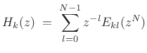 |
(12.49) |
or
![$\displaystyle \underbrace{\left[\begin{array}{c} H_0(z) \\ [2pt] H_1(z) \\ [2pt] \vdots \\ [2pt] \!\!H_{N-1}(z)\!\!\end{array}\right]}_{\bold{h}(z)} = \underbrace{\left[\begin{array}{cccc} E_{0,0}(z^N) & E_{0,1}(z^N) & \cdots & E_{0,N-1}(z^N) \\ E_{1,0}(z^N) & E_{1,1}(z^N) & \cdots & E_{1,N-1}(z^N)\\ \vdots & \vdots & \cdots & \vdots\\ \!\!E_{N-1,0}(z^N) & E_{N-1,1}(z^N) & \cdots & E_{N-1,N-1}(z^N) \!\! \end{array}\right]}_{\bold{E}(z^N)} \underbrace{\left[\begin{array}{c} 1 \\ [2pt] z^{-1} \\ [2pt] \vdots \\ [2pt] \!\!z^{-(N-1)}\!\!\end{array}\right]}_{\bold{e}(z)}$](http://www.dsprelated.com/josimages_new/sasp2/img2099.png) |
(12.50) |
which we can write as
| (12.51) |
Similarly, expand the synthesis filters in a type II polyphase decomposition:
 |
(12.52) |
or
![$\displaystyle \underbrace{\left[\begin{array}{c} F_0(z) \\ [2pt] F_1(z) \\ [2pt] \vdots \\ [2pt] \!\!F_{N-1}(z)\!\!\end{array}\right]^T}_{\bold{f}^T(z)} \eqsp \underbrace{\left[\begin{array}{c} \!\!z^{-(N-1)}\!\! \\ [2pt] \!\!z^{-(N-2)}\!\! \\ [2pt] \vdots \\ [2pt] 1\end{array}\right]^T}_{{\tilde{\bold{e}}}(z)} \underbrace{\left[\begin{array}{cccc} R_{0,0}(z^N) & R_{0,1}(z^N) & \cdots & R_{0,N-1}(z^N) \\ R_{1,0}(z^N) & R_{1,1}(z^N) & \cdots & R_{1,N-1}(z^N)\\ \vdots & \vdots & \cdots & \vdots\\ \!\!R_{N-1,0}(z^N) & R_{N-1,1}(z^N) & \cdots & R_{N-1,N-1}(z^N)\!\! \end{array}\right]}_{\bold{R}(z^N)}$](http://www.dsprelated.com/josimages_new/sasp2/img2102.png) |
(12.53) |
which we can write as
| (12.54) |
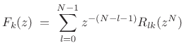
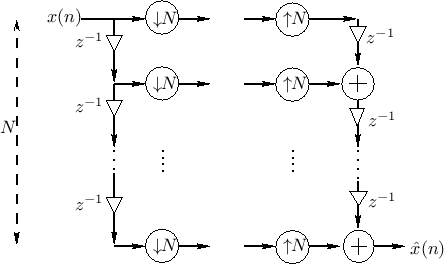
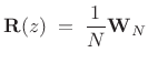
The polyphase representation can now be depicted as shown in
Fig.11.21. When ![]() , commuting the up/downsamplers gives
the result shown in Fig.11.22. We call
, commuting the up/downsamplers gives
the result shown in Fig.11.22. We call
![]() the
polyphase matrix.
the
polyphase matrix.
![\includegraphics[width=\twidth]{eps/polyNchan}](http://www.dsprelated.com/josimages_new/sasp2/img2105.png)
![\includegraphics[width=\twidth]{eps/polyNchanfast}](http://www.dsprelated.com/josimages_new/sasp2/img2106.png)
As we will show below, the above simplification can be carried out
more generally whenever ![]() divides
divides ![]() (e.g.,
(e.g.,
![]() ). In these cases
). In these cases
![]() becomes
becomes
![]() and
and
![]() becomes
becomes
![]() .
.
Simple Examples of Perfect Reconstruction
If we can arrange to have
| (12.55) |
then the filter bank will reduce to the simple system shown in Fig.11.23.
Thus, when ![]() and
and
![]() ,
we have a simple parallelizer/serializer,
which is perfect-reconstruction by inspection: Referring to
Fig.11.23, think of the input samples
,
we have a simple parallelizer/serializer,
which is perfect-reconstruction by inspection: Referring to
Fig.11.23, think of the input samples ![]() as ``filling'' a
length
as ``filling'' a
length ![]() delay line over
delay line over ![]() sample clocks. At time 0
, the
downsamplers and upsamplers ``fire'', transferring
sample clocks. At time 0
, the
downsamplers and upsamplers ``fire'', transferring ![]() (and
(and ![]() zeros) from the delay line to the output delay chain, summing with
zeros. Over the next
zeros) from the delay line to the output delay chain, summing with
zeros. Over the next ![]() clocks,
clocks, ![]() makes its way toward the
output, and zeros fill in behind it in the output delay chain.
Simultaneously, the input buffer is being filled with samples of
makes its way toward the
output, and zeros fill in behind it in the output delay chain.
Simultaneously, the input buffer is being filled with samples of
![]() . At time
. At time ![]() ,
, ![]() makes it to the output. At time
makes it to the output. At time ![]() ,
the downsamplers ``fire'' again, transferring a length
,
the downsamplers ``fire'' again, transferring a length ![]() ``buffer''
[
``buffer''
[![]() :
:![]() ] to the upsamplers. On the same clock pulse, the
upsamplers also ``fire'', transferring
] to the upsamplers. On the same clock pulse, the
upsamplers also ``fire'', transferring ![]() samples to the output delay
chain. The bottom-most sample [
samples to the output delay
chain. The bottom-most sample [
![]() ] goes out immediately
at time
] goes out immediately
at time ![]() . Over the next
. Over the next ![]() sample clocks, the length
sample clocks, the length ![]() output buffer will be ``drained'' and refilled by zeros.
Simultaneously, the input buffer will be replaced by new samples of
output buffer will be ``drained'' and refilled by zeros.
Simultaneously, the input buffer will be replaced by new samples of
![]() . At time
. At time ![]() , the downsamplers and upsamplers ``fire'', and
the process goes on, repeating with period
, the downsamplers and upsamplers ``fire'', and
the process goes on, repeating with period ![]() . The output of the
. The output of the
![]() -way parallelizer/serializer is therefore
-way parallelizer/serializer is therefore
| (12.56) |
and we have perfect reconstruction.
Sliding Polyphase Filter Bank
When ![]() , there is no downsampling or upsampling, and the system
further reduces to the case shown in Fig.11.24. Working
backward along the output delay chain, the output sum can be written
as
, there is no downsampling or upsampling, and the system
further reduces to the case shown in Fig.11.24. Working
backward along the output delay chain, the output sum can be written
as
![\begin{eqnarray*}
\hat{X}(z) &=& \left[z^{-0}z^{-(N-1)} + z^{-1}z^{-(N-2)} + z^{-2}z^{-(N-3)} + \cdots \right.\\
& & \left. + z^{-(N-2)}z^{-1} + z^{-(N-1)}z^{-0} \right] X(z)\\
&=& N z^{-(N-1)} X(z).
\end{eqnarray*}](http://www.dsprelated.com/josimages_new/sasp2/img2121.png)
Thus, when ![]() , the output is
, the output is
| (12.57) |
and we again have perfect reconstruction.
Hopping Polyphase Filter Bank
When ![]() and
and ![]() divides
divides ![]() , we have, by a similar analysis,
, we have, by a similar analysis,
 |
(12.58) |
which is again perfect reconstruction. Note the built-in overlap-add when
Sufficient Condition for Perfect Reconstruction
Above, we found that, for any integer
![]() which divides
which divides
![]() , a sufficient condition for perfect reconstruction is
, a sufficient condition for perfect reconstruction is
 |
(12.59) |
and the output signal is then
 |
(12.60) |
More generally, we allow any nonzero scaling and any additional delay:
where
 |
(12.62) |
Thus, given any polyphase matrix
![]() , we can attempt to compute
, we can attempt to compute
![]() : If it is stable, we can use it to build a
perfect-reconstruction filter bank. However, if
: If it is stable, we can use it to build a
perfect-reconstruction filter bank. However, if
![]() is FIR,
is FIR,
![]() will typically be IIR. In §11.5 below, we will look at
paraunitary filter banks, for which
will typically be IIR. In §11.5 below, we will look at
paraunitary filter banks, for which
![]() is FIR and
paraunitary whenever
is FIR and
paraunitary whenever
![]() is.
is.
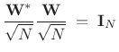
Necessary and Sufficient Conditions for Perfect Reconstruction
It can be shown [287] that the most general conditions for perfect reconstruction are that
![$\displaystyle \zbox {\bold{R}(z)\bold{E}(z) \eqsp c z^{-K} \left[\begin{array}{cc} \bold{0}_{(N-L)\times L} & z^{-1}\bold{I}_{N-L} \\ [2pt] \bold{I}_L & \bold{0}_{L \times (N-L)} \end{array}\right]}$](http://www.dsprelated.com/josimages_new/sasp2/img2132.png) |
(12.63) |
for some constant
Note that the more general form of
![]() above can be regarded as a (non-unique) square root of a vector unit delay, since
above can be regarded as a (non-unique) square root of a vector unit delay, since
![$\displaystyle \left[\begin{array}{cc} \bold{0}_{(N-L)\times L} & z^{-1}\bold{I}_{N-L} \\ [2pt] \bold{I}_L & \bold{0}_{L \times (N-L)} \end{array}\right]^2 \eqsp z^{-1}\bold{I}_N.$](http://www.dsprelated.com/josimages_new/sasp2/img2136.png) |
(12.64) |
Thus, the general case is the same thing as
| (12.65) |
except for some channel swapping and an extra sample of delay in some channels.
Polyphase View of the STFT
As a familiar special case, set
| (12.66) |
where
![$\displaystyle \bold{W}_N^\ast[kn] \eqsp \left[e^{-j2\pi kn/N}\right]$](http://www.dsprelated.com/josimages_new/sasp2/img2140.png) |
(12.67) |
The inverse of this polyphase matrix is then simply the inverse DFT matrix:
 |
(12.68) |
Thus, the STFT (with rectangular window) is the simple special case of a perfect reconstruction filter bank for which the polyphase matrix is constant. It is also unitary; therefore, the STFT is an orthogonal filter bank.
The channel analysis and synthesis filters are, respectively,
![\begin{eqnarray*}
H_k(z) &=& H_0(zW_N^k)\\ [5pt]
F_k(z) &=& F_0(zW_N^{-k})
\end{eqnarray*}](http://www.dsprelated.com/josimages_new/sasp2/img2142.png)
where
 , and
, and
![$\displaystyle F_0(z)\eqsp H_0(z)\eqsp \sum_{n=0}^{N-1}z^{-n}\;\longleftrightarrow\;[1,1,\ldots,1]$](http://www.dsprelated.com/josimages_new/sasp2/img2144.png) |
(12.69) |
corresponding to the rectangular window.
![\includegraphics[width=\twidth]{eps/polyNchanSTFT}](http://www.dsprelated.com/josimages_new/sasp2/img2145.png)
Looking again at the polyphase representation of the ![]() -channel
filter bank with hop size
-channel
filter bank with hop size ![]() ,
,
![]() ,
,
![]() ,
,
![]() dividing
dividing ![]() , we have the system shown in Fig.11.25.
Following the same analysis as in §11.4.1 leads to the following
conclusion:
, we have the system shown in Fig.11.25.
Following the same analysis as in §11.4.1 leads to the following
conclusion:
Our analysis showed that the STFT using a rectangular window is
a perfect reconstruction filter bank for all
integer hop sizes in the set
![]() .
The same type of analysis can be applied to the STFT using the other
windows we've studied, including Portnoff windows.
.
The same type of analysis can be applied to the STFT using the other
windows we've studied, including Portnoff windows.
Example: Polyphase Analysis of the STFT with 50% Overlap, Zero-Padding, and a Non-Rectangular Window
![\includegraphics[width=\twidth]{eps/polyNchanWinZPSTFT}](http://www.dsprelated.com/josimages_new/sasp2/img2150.png)
Figure 11.26 illustrates how a window and a hop size other than
![]() can be introduced into the polyphase representation of the STFT.
The constant-overlap-add of the window
can be introduced into the polyphase representation of the STFT.
The constant-overlap-add of the window ![]() is implemented in the
synthesis delay chain (which is technically the
transpose of a tapped delay
line). The downsampling factor and window must be selected
together to give constant overlap-add, independent of the
choice of polyphase matrices
is implemented in the
synthesis delay chain (which is technically the
transpose of a tapped delay
line). The downsampling factor and window must be selected
together to give constant overlap-add, independent of the
choice of polyphase matrices
![]() and
and
![]() (shown here as the
(shown here as the
![]() and
and
![]() ).
).
Example: Polyphase Analysis of the Weighted Overlap Add Case: 50% Overlap, Zero-Padding, and a Non-Rectangular Window
We may convert the previous example to a weighted overlap-add
(WOLA) (§8.6) filter bank by replacing each ![]() by
by
![]() and introducing these gains also between the
and introducing these gains also between the
![]() and
upsamplers, as shown in Fig.11.27.
and
upsamplers, as shown in Fig.11.27.
![\includegraphics[width=\twidth]{eps/polyNchanWinZPWOLA}](http://www.dsprelated.com/josimages_new/sasp2/img2155.png)
Paraunitary Filter Banks
Paraunitary filter banks form an interesting subset of perfect
reconstruction (PR) filter banks. We saw above that we get a PR filter
bank whenever the
synthesis polyphase matrix
![]() times the
analysis polyphase matrix
times the
analysis polyphase matrix
![]() is the identity matrix
is the identity matrix ![]() , i.e., when
, i.e., when
 |
(12.70) |
In particular, if
Paraconjugation is the generalization of the complex conjugate
transpose operation from the unit circle to the entire ![]() plane. A
paraunitary filter bank is therefore a generalization of an
orthogonal filter bank. Recall that an orthogonal filter bank
is one in which
plane. A
paraunitary filter bank is therefore a generalization of an
orthogonal filter bank. Recall that an orthogonal filter bank
is one in which
![]() is an orthogonal (or unitary) matrix, to
within a constant scale factor, and
is an orthogonal (or unitary) matrix, to
within a constant scale factor, and
![]() is its transpose (or
Hermitian transpose).
is its transpose (or
Hermitian transpose).
Lossless Filters
To motivate the idea of paraunitary filters, let's first review some properties of lossless filters, progressing from the simplest cases up to paraunitary filter banks:
A linear, time-invariant filter ![]() is said to be
lossless (or
allpass) if it preserves signal
energy. That is, if the input signal is
is said to be
lossless (or
allpass) if it preserves signal
energy. That is, if the input signal is ![]() , and the output
signal is
, and the output
signal is
![]() , then we have
, then we have
 |
(12.71) |
In terms of the
| (12.72) |
Notice that only stable filters can be lossless since, otherwise,
It is straightforward to show that losslessness implies
| (12.73) |
That is, the frequency response must have magnitude 1 everywhere on the unit circle in the
| (12.74) |
and this form generalizes to
The paraconjugate of a transfer function may be defined as the
analytic continuation of the complex conjugate from the unit circle to
the whole ![]() plane:
plane:
 |
(12.75) |
where
 |
(12.76) |
in which the conjugation of
We refrain from conjugating ![]() in the definition of the paraconjugate
because
in the definition of the paraconjugate
because
![]() is not analytic in the complex-variables sense.
Instead, we invert
is not analytic in the complex-variables sense.
Instead, we invert ![]() , which is analytic, and which
reduces to complex conjugation on the unit circle.
, which is analytic, and which
reduces to complex conjugation on the unit circle.
The paraconjugate may be used to characterize allpass filters as follows:
A causal, stable, filter ![]() is allpass if and only if
is allpass if and only if
| (12.77) |
Note that this is equivalent to the previous result on the unit circle since
| (12.78) |
To generalize lossless filters to the multi-input, multi-output (MIMO) case, we must generalize conjugation to MIMO transfer function matrices.
A ![]() transfer function matrix
transfer function matrix
![]() is
said to be lossless
if it is stable and its frequency-response matrix
is
said to be lossless
if it is stable and its frequency-response matrix
![]() is
unitary. That is,
is
unitary. That is,
| (12.79) |
for all
 |
(12.80) |
Note that
![]() is a
is a ![]() matrix
product of a
matrix
product of a ![]() times a
times a ![]() matrix. If
matrix. If ![]() , then
the rank must be deficient. Therefore, we must have
, then
the rank must be deficient. Therefore, we must have ![]() .
(There must be at least as many outputs as there are inputs, but it's
ok to have extra outputs.)
.
(There must be at least as many outputs as there are inputs, but it's
ok to have extra outputs.)
A lossless ![]() transfer function matrix
transfer function matrix
![]() is paraunitary,
i.e.,
is paraunitary,
i.e.,
| (12.81) |
Thus, every paraunitary matrix transfer function is unitary on the unit circle for all
Lossless Filter Examples
The simplest lossless filter is a unit-modulus gain
| (12.82) |
where
A lossless FIR filter can only consist of a single nonzero tap:
for some fixed integer
Every finite-order, single-input, single-output (SISO), lossless IIR filter (recursive allpass filter) can be written as
 |
(12.84) |
where
 . The polynomial
The normalized DFT matrix is an ![]() order zero paraunitary
transformation. This is because the normalized DFT matrix,
order zero paraunitary
transformation. This is because the normalized DFT matrix,
![]() ,
,
![]() , where
, where
![]() , is a unitary matrix:
, is a unitary matrix:
 |
(12.85) |
Properties of Paraunitary Filter Banks
Paraunitary systems are essentially multi-input, multi-output (MIMO)
allpass filters. Let
![]() denote the
denote the ![]() matrix transfer
function of a paraunitary system. In the square case (
matrix transfer
function of a paraunitary system. In the square case (![]() ), the
matrix determinant,
), the
matrix determinant,
![]() , is an allpass filter.
Therefore, if a square
, is an allpass filter.
Therefore, if a square
![]() contains FIR elements, its determinant
is a simple delay:
contains FIR elements, its determinant
is a simple delay:
![]() for some integer
for some integer ![]() .
.
An ![]() -channel analysis filter bank can be viewed as an
-channel analysis filter bank can be viewed as an ![]() MIMO filter:
MIMO filter:
![$\displaystyle \bold{H}(z) \eqsp \left[\begin{array}{c} H_1(z) \\ [2pt] H_2(z) \\ [2pt] \vdots \\ [2pt] H_N(z)\end{array}\right]$](http://www.dsprelated.com/josimages_new/sasp2/img2206.png) |
(12.86) |
A paraunitary filter bank must therefore satisfy
| (12.87) |
More generally, we allow paraunitary filter banks to scale and/or delay the input signal:
| (12.88) |
where
We can note the following properties of paraunitary filter banks:
- The synthesis filter bank is simply the paraconjugate of the
analysis filter bank:

(12.89)
That is, since the paraconjugate is the inverse of a paraunitary filter matrix, it is exactly what we need for perfect reconstruction. - The channel filters
 are power complementary:
(12.90)
This follows immediately from looking at the paraunitary property on the unit circle. - When
 is FIR, the corresponding synthesis filter matrix
 is also FIR.
- When
is FIR, each synthesis filter,
 , is simply the
 of its corresponding
analysis filter
of its corresponding
analysis filter
 :
:
(12.91)
where is the filter length. (When the filter coefficients are
complex,
includes a complex conjugation as well.) This
follows from the fact that paraconjugating an FIR filter amounts to
simply flipping (and conjugating) its coefficients. As we observed in
(11.83) above (§11.5.2), only trivial FIR filters of
the form
is the filter length. (When the filter coefficients are
complex,
includes a complex conjugation as well.) This
follows from the fact that paraconjugating an FIR filter amounts to
simply flipping (and conjugating) its coefficients. As we observed in
(11.83) above (§11.5.2), only trivial FIR filters of
the form
 can be paraunitary in the
single-input, single-output (SISO) case. In the MIMO case, on the
other hand, paraunitary systems can be composed of FIR filters of any
order.
can be paraunitary in the
single-input, single-output (SISO) case. In the MIMO case, on the
other hand, paraunitary systems can be composed of FIR filters of any
order.
- FIR analysis and synthesis filters in paraunitary filter banks
have the same amplitude response. This follows from the fact
that
 , i.e., flipping an FIR filter
impulse response
, i.e., flipping an FIR filter
impulse response  conjugates the frequency response, which does
not affect its amplitude response
conjugates the frequency response, which does
not affect its amplitude response
 .
.
- The polyphase matrix
 for any FIR paraunitary perfect
reconstruction filter bank can be written as the product of a
paraunitary and a unimodular matrix, where a
unimodular polynomial matrix
for any FIR paraunitary perfect
reconstruction filter bank can be written as the product of a
paraunitary and a unimodular matrix, where a
unimodular polynomial matrix
 is any square
polynomial matrix having a constant nonzero
determinant. For example,
is any square
polynomial matrix having a constant nonzero
determinant. For example, ![$\displaystyle \bold{U}(z) \eqsp
\left[\begin{array}{cc} 1+z^3 & z^2 \\ [2pt] z & 1 \end{array}\right] $](http://www.dsprelated.com/josimages_new/sasp2/img2221.png)
is unimodular. See [287, p. 663] for further details.
Examples
Consider the Haar filter bank discussed in §11.3.3, for which
![$\displaystyle \bold{H}(z) \eqsp \frac{1}{\sqrt{2}}\left[\begin{array}{c} 1+z^{-1} \\ [2pt] 1-z^{-1} \end{array}\right].$](http://www.dsprelated.com/josimages_new/sasp2/img2222.png) |
(12.92) |
The paraconjugate of
![$\displaystyle {\tilde {\bold{H}}}(z) \eqsp \frac{1}{\sqrt{2}}\left[\begin{array}{cc} 1+z & 1 - z \end{array}\right]$](http://www.dsprelated.com/josimages_new/sasp2/img2223.png) |
(12.93) |
so that
![$\displaystyle {\tilde {\bold{H}}}(z) \bold{H}(z) \eqsp \frac{1}{2} \left[\begin{array}{cc} 1+z & 1 - z \end{array}\right] \left[\begin{array}{c} 1+z^{-1} \\ [2pt] 1-z^{-1} \end{array}\right] \eqsp 1.$](http://www.dsprelated.com/josimages_new/sasp2/img2224.png) |
(12.94) |
Thus, the Haar filter bank is paraunitary. This is true for any power-complementary filter bank, since when
Filter Banks Equivalent to STFTs
We now turn to various practical examples of perfect reconstruction filter banks, with emphasis on those using FFTs in their implementation (i.e., various STFT filter banks).
Figure 11.28 illustrates a generic filter bank with ![]() channels,
much like we derived in §9.3.
The analysis filters
channels,
much like we derived in §9.3.
The analysis filters ![]() ,
,
![]() are bandpass filters
derived from a lowpass prototype
are bandpass filters
derived from a lowpass prototype ![]() by modulation (e.g.,
by modulation (e.g.,
 ), as
shown in the right portion of the figure. The channel signals
), as
shown in the right portion of the figure. The channel signals
![]() are given by the convolution of the input signal with
the
are given by the convolution of the input signal with
the ![]() th channel impulse response:
th channel impulse response:
From Chapter 9, we recognize this expression as the sliding-window STFT, where
![\begin{psfrags}
% latex2html id marker 30457\psfrag{z^-1}{{\large $z^{-1}$}}\psfrag{X(z)}{{\large $X(z)$}}\psfrag{X0(z)}{{\large $X_0(z)$}}\psfrag{X1(z)}{{\large $X_1(z)$}}\psfrag{X2(z)}{{\large $X_2(z)$}}\psfrag{Xn[0]}{{\normalsize $X_n(\omega_0)$}}\psfrag{Xn[1]}{{\normalsize $X_n(\omega_1)$}}\psfrag{Xn[2]}{{\normalsize $X_n(\omega_2)$}}\psfrag{H0(z)}{{\large $H_0(z)$}}\psfrag{H1(z)}{{\large $H_1(z)$}}\psfrag{H2(z)}{{\large $H_2(z)$}}\psfrag{W(-0n,N)}{{\small $W_N^{0n}$}}\psfrag{W(-1n,N)}{{\small $W_N^{-1n}$}}\psfrag{W(-2n,N)}{{\small $W_N^{-2n}$}}\psfrag{W(0n,N)}{{\small $W_N^{0n}$}}\psfrag{W(1n,N)}{{\small $W_N^{1n}$}}\psfrag{W(2n,N)}{{\small $W_N^{2n}$}}\psfrag{STFT}{}\begin{figure}[htbp]
\includegraphics[width=\twidth]{eps/portnoff}
\caption{Portnoff analysis bank for $N=3$.}
\end{figure}
\end{psfrags}](http://www.dsprelated.com/josimages_new/sasp2/img2233.png)
Suppose the analysis window ![]() (flip of the baseband-filter impulse
response
(flip of the baseband-filter impulse
response ![]() ) is length
) is length ![]() . Then in the context of overlap-add
processors (Chapter 8),
. Then in the context of overlap-add
processors (Chapter 8), ![]() is a Portnoff
window, and implementing the window with a length
is a Portnoff
window, and implementing the window with a length ![]() FFT requires
that the windowed data frame be time-aliased down to length
FFT requires
that the windowed data frame be time-aliased down to length
![]() prior to taking a length
prior to taking a length ![]() FFT (see §9.7). We can
obtain this same result via polyphase analysis, as elaborated in the
next section.
FFT (see §9.7). We can
obtain this same result via polyphase analysis, as elaborated in the
next section.
Polyphase Analysis of Portnoff STFT
Consider the ![]() th filter-bank channel filter
th filter-bank channel filter
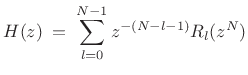
| (12.96) |
The impulse-response
![\begin{eqnarray*}
H_{0}(z) & = & \sum_{l=0}^{N-1} z^{-l}E_l(z^{N}) \\ [5pt]
H_{k}(z) & = & \sum_{l=0}^{N-1} (zW_N^k)^{-l} E_l[(z W_N^k)^{N}] \\ [5pt]
& = & \sum_{l=0}^{N-1} z^{-l} E_l(z^{N}) W_N^{-kl}.
\end{eqnarray*}](http://www.dsprelated.com/josimages_new/sasp2/img2238.png)
Consequently,
![\begin{eqnarray*}
H_{k}(z)X(z) & = & \sum_{l=0}^{N-1} z^{-l} E_l(z^{N})X(z) W_N^{-kl} \\
\left[\begin{array}{c}
H_{0}(z) \\
\ldots \\
H_{N-1}(z) \end{array} \right]
& = & \left[\begin{array}{ccc}
& & \\
& W_N^{-kl} & \\
& & \end{array} \right]
\left[\begin{array}{c}
E_0(z^N) z^{-0} X(z) \\
\ldots \\
E_{N-1}(z^N) z^{-(N-1)} X(z) \end{array}
\right].
\end{eqnarray*}](http://www.dsprelated.com/josimages_new/sasp2/img2239.png)
If ![]() is a good
is a good ![]() th-band lowpass, the subband signals
th-band lowpass, the subband signals
![]() are bandlimited to a region of width
are bandlimited to a region of width ![]() . As a result,
there is negligible aliasing when we downsample each of the subbands
by
. As a result,
there is negligible aliasing when we downsample each of the subbands
by ![]() . Commuting the downsamplers to get an efficient implementation
gives Fig.11.29.
. Commuting the downsamplers to get an efficient implementation
gives Fig.11.29.
![\begin{psfrags}
% latex2html id marker 30545\psfrag{X(z)}{{\large $X(z)$}}\psfrag{E0(z^3)}{{\large $E_0(z^3)$}}\psfrag{E1(z^3)}{{\large $E_1(z^3)$}}\psfrag{E2(z^3)}{{\large $E_2(z^3)$}}\psfrag{E0(z)}{{\large $E_0(z)$}}\psfrag{E1(z)}{{\large $E_1(z)$}}\psfrag{E2(z)}{{\large $E_2(z)$}}\psfrag{X0(z)}{{\large $X_0(z)$}}\psfrag{X1(z)}{{\large $X_1(z)$}}\psfrag{X2(z)}{{\large $X_2(z)$}}\begin{figure}[htbp]
\includegraphics[width=\twidth]{eps/polystft}
\caption{Polyphase implementation of
Portnoff STFT filter bank for $N=3$.}
\end{figure}
\end{psfrags}](http://www.dsprelated.com/josimages_new/sasp2/img2241.png)
First note that if
![]() for all
for all ![]() , the system of
Fig.11.29 reduces to a rectangularly windowed STFT in which the
window length
, the system of
Fig.11.29 reduces to a rectangularly windowed STFT in which the
window length ![]() equals the DFT length
equals the DFT length ![]() . The downsamplers
``hold off'' the DFT until the length 3 delay line fills with new
input samples, then it ``fires'' to produce a spectral frame. A new
spectral frame is produced after every third sample of input data is
received.
. The downsamplers
``hold off'' the DFT until the length 3 delay line fills with new
input samples, then it ``fires'' to produce a spectral frame. A new
spectral frame is produced after every third sample of input data is
received.
In the more general case in which ![]() are nontrivial filters,
such as
are nontrivial filters,
such as
![]() , for example, they can be seen to compute the
equivalent of a time aliased windowed input frame, such as
, for example, they can be seen to compute the
equivalent of a time aliased windowed input frame, such as
![]() . This follows because the filters operate on the
downsampled input stream, so that the filter coefficients operate on
signal samples separated by
. This follows because the filters operate on the
downsampled input stream, so that the filter coefficients operate on
signal samples separated by ![]() samples. The linear combination of
these samples by the filter implements the time-aliased windowed data
frame in a Portnoff-windowed overlap-add STFT. Taken together, the
polyphase filters
samples. The linear combination of
these samples by the filter implements the time-aliased windowed data
frame in a Portnoff-windowed overlap-add STFT. Taken together, the
polyphase filters ![]() compute the appropriately time-aliased data
frame windowed by
compute the appropriately time-aliased data
frame windowed by
![]() .
.
In the overlap-add interpretation of Fig.11.29, the window is
hopped by ![]() samples. While this was the entire window length in
the rectangular window case (
samples. While this was the entire window length in
the rectangular window case (![]() ), it is only a portion of the
effective frame length
), it is only a portion of the
effective frame length ![]() when the analysis filters have order 1 or
greater.
when the analysis filters have order 1 or
greater.
MPEG Filter Banks
This section provides some highlights of the history of filter banks used for perceptual audio coding (MPEG audio). For a more complete introduction and discussion of MPEG filter banks, see, e.g., [16,273].
Pseudo-QMF Cosine Modulation Filter Bank
Section 11.3.5 introduced two-channel quadrature mirror filter banks (QMF). QMFs were shown to provide a particular class of perfect reconstruction filter banks. We found, however, that the quadrature mirror constraint on the analysis filters,
| (12.97) |
was rather severe in that linear-phase FIR implementations only exist in the two-tap case
The Pseudo-QMF (PQMF) filter bank is a ``near perfect
reconstruction'' filter bank in which aliasing cancellation occurs
only between adjacent bands [194,287]. The PQMF
filters commonly used in perceptual audio coders employ bandpass
filters with stop-band attenuation near ![]() dB, so the neglected
bands (which alias freely) are not significant. An outline of the
design procedure is as follows:
dB, so the neglected
bands (which alias freely) are not significant. An outline of the
design procedure is as follows:
- Design a lowpass prototype window,
, with length
 ,
,
- The lowpass design is
constrained to give aliasing cancellation in neighboring subbands:
- The filter bank analysis filters
 are cosine modulations of
:
are cosine modulations of
:
![$\displaystyle h_k(n) \eqsp h(n)\hbox{cos}\left[\left(k+\frac{1}{2}\right)\left(n-\frac{M-1}{2}\right)\frac{\pi}{N} + \phi_k\right],$](http://www.dsprelated.com/josimages_new/sasp2/img2254.png)
(12.98)
 , where the phases are restricted according to
(12.99)
again for aliasing cancellation. - Since it is an orthogonal filter bank by construction,
the synthesis filters are simply the time-reverse of the analysis filters:
(12.100)
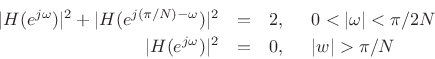
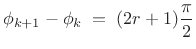
Perfect Reconstruction Cosine Modulated Filter Banks
By changing the phases ![]() , the pseudo-QMF filter bank can yield
perfect reconstruction:
, the pseudo-QMF filter bank can yield
perfect reconstruction:
 |
(12.101) |
where
If ![]() , then this is the
oddly stacked Princen-Bradley filter bank
and the analysis filters are related by cosine modulations of
the lowpass prototype:
, then this is the
oddly stacked Princen-Bradley filter bank
and the analysis filters are related by cosine modulations of
the lowpass prototype:
![$\displaystyle f_k(n) \eqsp h(n)\hbox{cos}\left[\left(n+\frac{N+1}{2}\right)\left(k+\frac{1}{2}\right)\frac{\pi}{N}\right],\quad k=0,\ldots,N-1$](http://www.dsprelated.com/josimages_new/sasp2/img2262.png) |
(12.102) |
However, the length of the filters
| (12.103) |
The parameter
MPEG Layer III Filter Bank
MPEG 1 and 2, Layer III is popularly known as ``MP3 format.'' The original MPEG 1 and 2, Layers I and II, based on the MUSICAM coder, contained only 32 subbands, each band approximately 650 Hz wide, implemented using a length 512 lowpass-prototype window, lapped (``time aliased'') by factor of 512/32 = 16, thus yielding 32 real bands with 96 dB of stop-band rejection, and having a hop size of 32 samples [149, §4.1.1]. It was found, however, that a higher coding gain was obtained using a finer frequency resolution. As a result, the MPEG 1&2 Layer III coder (based on the ASPEC coder from AT&T), appended a Princen-Bradley filter bank [214] having 6 to 18 subbands to the output of each subband of the 32-channel PQMF cosine-modulated analysis filter bank [149, § 4.1.2]. The number of sub-bands and window shape were chosen to be signal-dependent as follows:
- Transients use
 subbands, corresponding to relatively
high time resolution and low frequency resolution.
subbands, corresponding to relatively
high time resolution and low frequency resolution.
- Steady-state tones use
 subbands, corresponding to higher
frequency resolution and lower time resolution relative to
transients.12.3
subbands, corresponding to higher
frequency resolution and lower time resolution relative to
transients.12.3
- The encoder generates a function called the perceptual entropy (PE) which tells the coder when to switch resolutions.
The MPEG AAC coder is often regarded as providing nearly twice the
compression ratio of ``MP3'' (MPEG 1-2 Layer III) coding at the same
quality level.12.4 MPEG AAC
introduced a new MDCT filter bank that adaptively switches between 128
and 1024 bands (length 256 and 2048 FFT windows, using 50% overlap)
[149, §4.1.6]. The nearly doubled number of frequency
bands available for coding steady-state signal intervals contributed
much to the increased coding gain of AAC over MP3. The 128-1024 MDCT
filter bank in AAC is also considerably simpler than the hierarchical
![]() -
-![]() MP3 filter bank, without requiring the ``cross-talk
aliasing reduction'' needed by the PQMF/MDCT hierarchical filter bank
of MP3 [149, §4.1.6].
MP3 filter bank, without requiring the ``cross-talk
aliasing reduction'' needed by the PQMF/MDCT hierarchical filter bank
of MP3 [149, §4.1.6].
The MPEG-4 audio compression standard (there was no MPEG-3), included a new transform coder based on the AAC filter bank [149, §4.1.7].
See, e.g., [16,273] for much more on MPEG coders and related topics. Chapter 4 of [149] contains an excellent summary of MPEG, Sony ATRAC, and Dolby AC-n coders up to 1998.
Review of STFT Filterbanks
Let's take a look at some of the STFT processors we've seen before, now viewed as polyphase filter banks. Since they all use FFTs to perform overlap-add decompositions of spectra, they are all efficient, but most are oversampled in time and/or frequency as ``filter banks'' go. Oversampling is usually preferred outside of a compression context, and normally required when spectral modifications are to be performed. The STFT also computes a uniform filter bank, but it can be used as the basis for a variety of non-uniform filter banks, as discussed in §10.7, to give frequency resolution more like that of hearing (§7.3).
For each selected STFT example below, a list of filter-bank properties
is listed, followed by some discussion. Most of the properties are
determined by the choice of FFT window ![]() and FFT hop size
and FFT hop size ![]() .
.
STFT, Rectangular Window, No Overlap
- Perfect reconstruction
- Critically sampled (relies on aliasing cancellation)
- Poor channel isolation (
 dB)
dB)
- Not robust to filter-bank modifications
STFT, Rectangular Window, 50% Overlap
- Perfect reconstruction
- Oversampled by 2 (less reliant on aliasing cancellation)
- Poor channel isolation (
dB)
- Not very robust to filter-bank modifications, but better
STFT, Triangular Window, 50% Overlap
- Perfect reconstruction
- Oversampled by 2
- Better channel isolation (
 dB)
dB)
- Moderately robust to filter-bank modifications
STFT, Hamming Window, 75% Overlap
- Perfect reconstruction
- Oversampled by 4
- Aliasing from side lobes only
- Good channel isolation (
 dB)
dB)
- Moderately robust to filter-bank modifications
STFT, Kaiser Window, Beta=10, 90% Overlap
- Approximate perfect reconstruction (side lobes controlled by
 )
)
- Oversampled by

- Excellent channel isolation (
 dB)
dB)
- Very robust to filter-bank modifications
- Aliasing from side lobes only
Sliding FFT (Maximum Overlap), Any Window, Zero-Padded by 5
- Perfect reconstruction (always true when hop-size
 )
)
- Oversampled by
 , where

 = window length (time-domain oversampling factor)
-
- 5 = zero-padding factor (frequency-domain oversampling factor)
- Excellent channel isolation (set by window side lobes)
- Extremely robust to filter-bank modifications
- No aliasing to cancel!
Wavelet Filter Banks
Let's now approach filter-bank derivation from a ``Hilbert space'' (geometric) point of view. This is the most natural setting for the study of wavelet filter banks [291,287].
Geometric Signal Theory
In general, signals can be expanded as a linear combination
of orthonormal basis signals ![]() [264]. In the
discrete-time case, this can be expressed as
[264]. In the
discrete-time case, this can be expressed as
where the coefficient of projection of
 |
(12.105) |
and the basis signals are orthonormal:
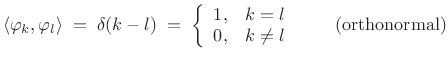 |
(12.106) |
The signal expansion (11.104) can be interpreted geometrically as a sum of orthogonal projections of
![\includegraphics[width=0.5\twidth]{eps/proj}](http://www.dsprelated.com/josimages_new/sasp2/img2285.png)
A set of signals
![]() is said to be
a biorthogonal basis set if any signal
is said to be
a biorthogonal basis set if any signal ![]() can be represented
as
can be represented
as
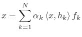 |
(12.107) |
where
The following examples illustrate the Hilbert space point of view for various familiar cases of the Fourier transform and STFT. A more detailed introduction appears in Book I [264].
Natural Basis
The natural basis for a discrete-time signal ![]() is the set
of shifted impulses:
is the set
of shifted impulses:
![$\displaystyle \varphi_k \isdefs [\ldots, 0,\underbrace{1}_{k^{\hbox{\tiny th}}},0,\ldots],$](http://www.dsprelated.com/josimages_new/sasp2/img2291.png) |
(12.108) |
or,
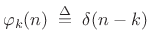 |
(12.109) |
for all integers
| (12.110) |
so that the expansion of
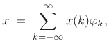 |
(12.111) |
i.e.,
 |
|||
 |
This expansion was used in Book II [263] to derive the impulse-response representation of an arbitrary linear, time-invariant filter.
Normalized DFT Basis for 
The Normalized Discrete Fourier Transform (NDFT) (introduced in
Book I [264]) projects the signal ![]() onto
onto ![]() discrete-time sinusoids of length
discrete-time sinusoids of length ![]() , where the sinusoids are
normalized to have unit
, where the sinusoids are
normalized to have unit ![]() norm:
norm:
 |
(12.112) |
and
 |
|||
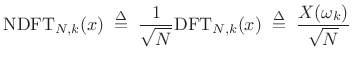 |
and the expansion of
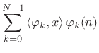 |
|||
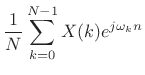 |
|||
for
Normalized Fourier Transform Basis
The Fourier transform projects a continuous-time signal ![]() onto an
infinite set of continuous-time complex sinusoids
onto an
infinite set of continuous-time complex sinusoids
![]() ,
for
,
for
![]() . These sinusoids all have infinite
. These sinusoids all have infinite ![]() norm, but a simple normalization by
norm, but a simple normalization by
![]() can be chosen so
that the inverse Fourier transform has the desired form of a
superposition of projections:
can be chosen so
that the inverse Fourier transform has the desired form of a
superposition of projections:
 |
(12.113) |
 |
|||
 |
|||
 |
|||
 |
|||
Normalized DTFT Basis
The Discrete Time Fourier Transform (DTFT) is similar to the Fourier transform case:
![$\displaystyle \varphi _\omega (n) \isdef e^{j\omega n}/\sqrt{2\pi},\quad \omega \in (-\pi,\pi], \quad n\in (-\infty,\infty)$](http://www.dsprelated.com/josimages_new/sasp2/img2317.png) |
(12.114) |
The inner product
Normalized STFT Basis
The Short Time Fourier Transform (STFT) is defined as a time-ordered
sequence of DTFTs, and implemented in practice as a sequence of FFTs
(see §7.1). Thus, the signal basis functions are naturally
defined as the DFT-sinusoids multiplied by time-shifted windows,
suitably normalized for unit ![]() norm:
norm:
 |
(12.115) |
![$\displaystyle \omega_k = \frac{2\pi k}{N}, \quad k \in [0,N-1], \quad n\in (-\infty,\infty),\quad w(n)\in{\cal R},$](http://www.dsprelated.com/josimages_new/sasp2/img2321.png) |
(12.116) |
and
When successive windows overlap (i.e., the hop size ![]() is less than
the window length
is less than
the window length ![]() ), the basis functions are not
orgthogonal. In this case, we may say that the basis set
is overcomplete.
), the basis functions are not
orgthogonal. In this case, we may say that the basis set
is overcomplete.
The basis signals are orthonormal when ![]() and the rectangular
window is used (
and the rectangular
window is used (![]() ). That is, two rectangularly windowed DFT
sinusoids are orthogonal when either the frequency bin-numbers or the
time frame-numbers differ, provided that the window length
). That is, two rectangularly windowed DFT
sinusoids are orthogonal when either the frequency bin-numbers or the
time frame-numbers differ, provided that the window length ![]() equals
the number of DFT frequencies
equals
the number of DFT frequencies ![]() (no zero padding). In other words,
we obtain an orthogonal basis set in the STFT when the hop size,
window length, and DFT length are all equal (in which case the
rectangular window must be used to retain the perfect-reconstruction
property). In this case, we can write
(no zero padding). In other words,
we obtain an orthogonal basis set in the STFT when the hop size,
window length, and DFT length are all equal (in which case the
rectangular window must be used to retain the perfect-reconstruction
property). In this case, we can write
| (12.117) |
i.e.,
![$\displaystyle \varphi_{mk}(n) = \left\{\begin{array}{ll} \frac{e^{j\omega_k n}}{\sqrt{N}}, & mN \leq n \leq (m+1)N-1 \\ [5pt] 0, & \mbox{otherwise.} \\ \end{array} \right.$](http://www.dsprelated.com/josimages_new/sasp2/img2324.png) |
(12.118) |
The coefficient of projection can be written
 |
|||
 |
so that the signal expansion can be interpreted as
 |
|||
 |
|||
![$\displaystyle \sum_{m=-\infty}^{\infty}
\hbox{\sc Shift}_{mN,n}\left\{\hbox{\sc ZeroPad}_\infty\left[\hbox{DFT}_N^{-1}(X_m)\right]\right\}$](http://www.dsprelated.com/josimages_new/sasp2/img2331.png) |
|||
In the overcomplete case, we get a special case of weighted
overlap-add (§8.6):
|
|||
 |
Continuous Wavelet Transform
In the present (Hilbert space) setting, we can now easily define the continuous wavelet transform in terms of its signal basis set:
 |
|||
 |
The parameter
![\includegraphics[width=0.8\twidth]{eps/wavelets}](http://www.dsprelated.com/josimages_new/sasp2/img2341.png)
The so-called admissibility condition for a mother wavelet
![]() is
is
Given sufficient decay with
The Morlet wavelet is simply a Gaussian-windowed complex sinusoid:
 |
|||
The scale factor is chosen so that
| (12.119) |
In this case, we have
Since the scale parameter of a wavelet transform is analogous to frequency in a Fourier transform, a wavelet transform display is often called a scalogram, in analogy with an STFT ``spectrogram'' (discussed in §7.2).
When the mother wavelet can be interpreted as a windowed sinusoid (such as the Morlet wavelet), the wavelet transform can be interpreted as a constant-Q Fourier transform.12.5Before the theory of wavelets, constant-Q Fourier transforms (such as obtained from a classic third-octave filter bank) were not easy to invert, because the basis signals were not orthogonal. See Appendix E for related discussion.
Discrete Wavelet Transform
The discrete wavelet transform is a discrete-time,
discrete-frequency counterpart of the continuous wavelet transform of
the previous section:
 |
|||
 |
where
The inverse transform is, as always, the signal expansion in terms of the orthonormal basis set:
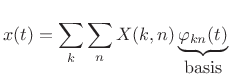 |
(12.120) |
We can show that discrete wavelet transforms are constant-Q by
defining the center frequency of the ![]() th basis signal as the
geometric mean of its bandlimits
th basis signal as the
geometric mean of its bandlimits ![]() and
and ![]() , i.e.,
, i.e.,
 |
(12.121) |
Then
 |
(12.122) |
which does not depend on
Discrete Wavelet Filterbank
In a discrete wavelet filterbank, each basis signal is
interpreted as the impulse response of a bandpass filter in a
constant-Q filter bank:
 |
|||
Thus, the
Recall that in the STFT, channel filter
![]() is a shift of
the zeroth channel-filter
is a shift of
the zeroth channel-filter
![]() (which corresponds to ``cosine
modulation'' in the time domain).
(which corresponds to ``cosine
modulation'' in the time domain).
As the channel-number ![]() increases, the channel impulse response
increases, the channel impulse response
![]() lengthens by the factor
lengthens by the factor ![]() ., while the pass-band of its
frequency-response
., while the pass-band of its
frequency-response ![]() narrows by the inverse factor
narrows by the inverse factor ![]() .
.
Figure 11.32 shows a block diagram of the discrete wavelet
filter bank for ![]() (the ``dyadic'' or ``octave filter-bank'' case),
and Fig.11.33 shows its time-frequency tiling as compared to
that of the STFT. The synthesis filters
(the ``dyadic'' or ``octave filter-bank'' case),
and Fig.11.33 shows its time-frequency tiling as compared to
that of the STFT. The synthesis filters ![]() may be used to make
a biorthogonal filter bank. If the
may be used to make
a biorthogonal filter bank. If the ![]() are orthonormal, then
are orthonormal, then
![]() .
.
![\includegraphics[width=\twidth]{eps/DyadicFilterbank}](http://www.dsprelated.com/josimages_new/sasp2/img2371.png)
![\includegraphics[width=0.8\twidth]{eps/DyadicTiling}](http://www.dsprelated.com/josimages_new/sasp2/img2372.png) |
Dyadic Filter Banks
![\includegraphics[width=0.7\twidth]{eps/dyadicFilters}](http://www.dsprelated.com/josimages_new/sasp2/img2373.png)
A dyadic filter bank is any octave filter
bank,12.6 as illustrated qualitatively in Figure 11.34. Note that
![]() is the top-octave bandpass filter,
is the top-octave bandpass filter,
![]() is the bandpass filter for next octave down,
is the bandpass filter for next octave down,
![]() is the octave bandpass below that, and so on. The optional
scale factors result in the same sum-of-squares for each
channel-filter impulse response.
is the octave bandpass below that, and so on. The optional
scale factors result in the same sum-of-squares for each
channel-filter impulse response.
A dyadic filter bank may be derived from the discrete wavelet filter
bank by setting ![]() and relaxing the exact orthonormality
requirement on the channel-filter impulse responses. If they do
happen to be orthonormal, we may call it a dyadic wavelet filter
bank.
and relaxing the exact orthonormality
requirement on the channel-filter impulse responses. If they do
happen to be orthonormal, we may call it a dyadic wavelet filter
bank.
For a dyadic filter bank, the center-frequency of the ![]() th
channel-filter impulse response can be defined as
th
channel-filter impulse response can be defined as
| (12.123) |
so that
 |
(12.124) |
Thus, a dyadic filter bank is a special case of a constant-Q filter bank for which the
Dyadic Filter Bank Design
Design of dyadic filter banks using the window method for FIR digital filter design (introduced in §4.5) is described in, e.g., [226, §6.2.3b].
A ``very easy'' method suggested in [287, §11.6] is to design a two-channel paraunitary QMF bank, and repeat recursively to split the lower-half of the spectrum down to some desired depth.
Generalized STFT
A generalized STFT may be defined by [287]
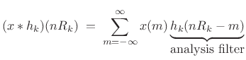 |
|||
 |
This filter bank and its reconstruction are diagrammed in Fig.11.35.
![\includegraphics[width=\twidth]{eps/GenSTFT}](http://www.dsprelated.com/josimages_new/sasp2/img2383.png)
The analysis filter ![]() is typically complex bandpass (as in the
STFT case). The integers
is typically complex bandpass (as in the
STFT case). The integers ![]() give the downsampling factor for the
output of the
give the downsampling factor for the
output of the ![]() th channel filter: For critical sampling without
aliasing, we set
th channel filter: For critical sampling without
aliasing, we set
![]() . The impulse response of
synthesis filter
. The impulse response of
synthesis filter ![]() can be regarded as the
can be regarded as the ![]() th basis
signal in the reconstruction. If the
th basis
signal in the reconstruction. If the ![]() are orthonormal, then
we have
are orthonormal, then
we have
![]() . More generally,
. More generally,
![]() form
a biorthogonal basis.
form
a biorthogonal basis.
Further Reading
In addition to [287] which was frequently cited in this chapter, [291], [160], [16], [273] are excellent references (books). The original paper by Princen and Bradley on time-domain aliasing cancellation is [214]. The Princen-Bradley filter bank is a special case of Lapped Orthogonal Transforms (LOT) [160] for which the overlap is 50%. It is also an orthogonal perfect reconstruction filter bank with first-order FIR polyphase filters. Other papers related to perceptual audio coding include [24,284,53,161,195,17,25,18,200,16,273]. An approximately invertible constant-Q transform, with FOSS matlab code, is described in [244].
Conclusions
This chapter introduced various multirate filter banks. While the main purpose was to relate them to STFT processors (which the author found to be missing in the literature), it is difficult to avoid being drawn into the general topic of perfect-reconstruction filter banks!
Next Section:
Summary and Conclusions
Previous Section:
Applications of the STFT


