


One Sine and One Cosine ``Phase Quadrature'' Case
Figure 5.8 shows a similar spectrum analysis of two sinusoids
| (6.18) |
using the same frequency separation and window lengths. However, now the sinusoids are 90 degrees out of phase (one sine and one cosine). Curiously, the top-left case (
![\includegraphics[width=\twidth]{eps/resolvedSinesB}](http://www.dsprelated.com/josimages_new/sasp2/img956.png)
Figure 5.9 shows the same plots as in Fig.5.8, but overlaid. From this we can see that the peak locations are biased in under-resolved cases, both in amplitude and frequency.
![\includegraphics[width=\textwidth ]{eps/resolvedSinesC2C}](http://www.dsprelated.com/josimages_new/sasp2/img957.png)
The preceding figures suggest that, for a rectangular window of length
![]() , two sinusoids are well resolved when they are separated in
frequency by
, two sinusoids are well resolved when they are separated in
frequency by
 |
(6.19) |
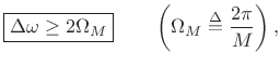
where the frequency-separation
 |
(6.20) |
where the
 denotes normalized frequency in
cycles per sample. In Hz, we have
denotes normalized frequency in
cycles per sample. In Hz, we have
 |
(6.21) |
or
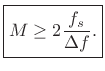 |
(6.22) |
Note that
A more detailed study [1] reveals that ![]() cycles
of the difference-frequency is sufficient to enable fully accurate
peak-frequency measurement under the rectangular window by means of
finding FFT peaks. In §5.5.2 below, additional minimum duration
specifications for resolving closely spaced sinusoids are given for
other window types as well.
cycles
of the difference-frequency is sufficient to enable fully accurate
peak-frequency measurement under the rectangular window by means of
finding FFT peaks. In §5.5.2 below, additional minimum duration
specifications for resolving closely spaced sinusoids are given for
other window types as well.
In principle, we can resolve arbitrarily small frequency separations, provided
- there is no noise, and
- we are sure we are looking at the sum of two ideal sinusoids under the window.
The rectangular window provides an abrupt transition at its edge. While it remains the optimal window for sinusoidal peak estimation, it is by no means optimal in all spectrum analysis and/or signal processing applications involving spectral processing. As discussed in Chapter 3, windows with a more gradual transition to zero have lower side-lobe levels, and this is beneficial for spectral displays and various signal processing applications based on FFT methods. We will encounter such applications in later chapters.
Next Section:
Phase Interpolation at a Peak
Previous Section:
Two Cosines (``In-Phase'' Case)


