STFT of COLA Decomposition

To represent practical implementations using the FFT, it is preferable to shift the $m^{th}$ frame back to the time origin:

$\displaystyle {\tilde x}_m(n) \isdef x_m(n+mR) = \hbox{\sc Shift}_{-mR,n}(x_m)$

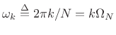
This is summarized in Fig.8.12. Zero-based frames are needed because the FFT always treats its leftmost input sample as occurring at time zero. In other words, a hopping FFT effectively redefines time zero on each hop. Thus, a practical STFT is a sequence of FFTs of the zero-based frames ${\tilde x}_0, {\tilde x}_1, \ldots$ . On the other hand, papers in the literature (such as [8,10]) work with the fixed time-origin case ( $x_0, x_1, \ldots$ ). Since they differ only by a time shift, it is not hard to translate back and forth.

$\begin{psfrags} % latex2html id marker 22017\psfrag{x}{$x$}\psfrag{Zero-cen... ... frame shifted to time 0, ${\tilde x}_3$\ (bottom).} \end{figure} \end{psfrags}$

Note that we may sample the DTFT of both and ${\tilde x}_m$ , because both are time-limited to nonzero samples. The minimum information-preserving sampling interval along the unit circle in both cases is $\Omega_M \isdeftext 2\pi/M$ . In practice, we often oversample to some extent, using $\Omega_N$ with instead. For ${\tilde x}_m$ , we get

$\displaystyle {\tilde X}_m(\omega_k)$	$\displaystyle \isdef$	$\displaystyle \hbox{\sc Sample}_{\Omega_N,k}\left(\hbox{\sc DTFT}\left({\tilde x}_m\right)\right)$
	$\displaystyle =$	$\displaystyle \hbox{\sc DFT}_{N,k}({\tilde x}_m), \protect$	(9.3)

where $\omega_k \isdef 2\pi k/N = k\Omega_N$ . For we have

$\begin{eqnarray*} X_m(\omega_k) &\isdef & \hbox{\sc Sample}_{\Omega_N,k}\left(\h... ...\sc Alias}_N(x_m)\\ &\neq& {\tilde x}_m \; \hbox{(in general).} \end{eqnarray*}$

Since ${\tilde x}_m = \hbox{\sc Shift}_{-mR}(x_m)$ , their transforms are related by the shift theorem:

$\begin{eqnarray*} {\tilde X}_m(\omega_k) &=& e^{jmR\omega_k} X_m(\omega_k) \\ \... ...de x}_m(n) &=& \hbox{\sc Alias}_{N,n+mR}(x_m)\\ &=& x_m(n+mR)_N \end{eqnarray*}$

where denotes modulo indexing (appropriate since the DTFTs have been sampled at intervals of $\Omega_N = 2\pi/N$ ).

Order a Hardcopy of Spectral Audio Signal Processing

Previous: COLA Examples
Next: Acyclic Convolution

written by Julius Orion Smith III
Julius Smith's background is in electrical engineering (BS Rice 1975, PhD Stanford 1983). He is presently Professor of Music and Associate Professor (by courtesy) of Electrical Engineering at Stanford's Center for Computer Research in Music and Acoustics (CCRMA), teaching courses and pursuing research related to signal processing applied to music and audio systems. See http://ccrma.stanford.edu/~jos/ for details.

Sign in

Search Online Books

Free Online Books

Sponsor

Chapters

Spectral Audio Signal Processing
    Overlap-Add (OLA) STFT Processing
       Convolving with Long Signals
          STFT of COLA Decomposition