


Sample-Variance Variance
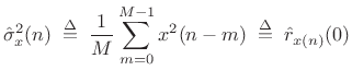
Consider now the sample variance estimator
 |
(C.33) |
where the mean is assumed to be
![$ {\cal E}\left\{[\hat{\sigma}_x^2(n)]^2\right\} = {\cal E}\left\{\hat{r}_{x(n)}^2(0)\right\} = \sigma_x^2$](http://www.dsprelated.com/josimages_new/sasp2/img2708.png) .
The variance of this estimator is then given by
.
The variance of this estimator is then given by
![\begin{eqnarray*}
\mbox{Var}\left\{\hat{\sigma}_x^2(n)\right\} &\isdef & {\cal E}\left\{[\hat{\sigma}_x^2(n)-\sigma_x^2]^2\right\}\\
&=& {\cal E}\left\{[\hat{\sigma}_x^2(n)]^2-\sigma_x^4\right\}
\end{eqnarray*}](http://www.dsprelated.com/josimages_new/sasp2/img2709.png)
where
![\begin{eqnarray*}
{\cal E}\left\{[\hat{\sigma}_x^2(n)]^2\right\} &=&
\frac{1}{M^2}\sum_{m_1=0}^{M-1}\sum_{m_1=0}^{M-1}{\cal E}\left\{x^2(n-m_1)x^2(n-m_2)\right\}\\
&=& \frac{1}{M^2}\sum_{m_1=0}^{M-1}\sum_{m_1=0}^{M-1}r_{x^2}(\vert m_1-m_2\vert)
\end{eqnarray*}](http://www.dsprelated.com/josimages_new/sasp2/img2710.png)
The autocorrelation of ![]() need not be simply related to that of
need not be simply related to that of
![]() . However, when
. However, when ![]() is assumed to be Gaussian white
noise, simple relations do exist. For example, when
is assumed to be Gaussian white
noise, simple relations do exist. For example, when
![]() ,
,
| (C.34) |
by the independence of
When ![]() is assumed to be Gaussian white noise, we have
is assumed to be Gaussian white noise, we have
![$\displaystyle {\cal E}\left\{x^2(n-m_1)x^2(n-m_2)\right\} = \left\{\begin{array}{ll} \sigma_x^4, & m_1\ne m_2 \\ [5pt] 3\sigma_x^4, & m_1=m_2 \\ \end{array} \right.$](http://www.dsprelated.com/josimages_new/sasp2/img2721.png) |
(C.35) |
so that the variance of our estimator for the variance of Gaussian white noise is
Var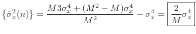 |
(C.36) |
Again we see that the variance of the estimator declines as
The same basic analysis as above can be used to estimate the variance of the sample autocorrelation estimates for each lag, and/or the variance of the power spectral density estimate at each frequency.
As mentioned above, to obtain a grounding in statistical signal processing, see references such as [201,121,95].
Next Section:
Uniform Distribution
Previous Section:
Sample-Mean Variance


