


Spectrum of a Sinusoid
A sinusoid is any signal of the form
| (6.1) |
where
By Euler's identity,
![]() , we can write
, we can write
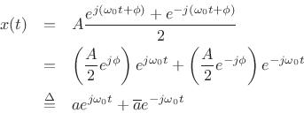
where
![]() denotes the complex conjugate of
denotes the complex conjugate of ![]() .
Thus, we can build a real sinusoid
.
Thus, we can build a real sinusoid ![]() as a linear combination of
positive- and negative-frequency complex sinusoidal components:
as a linear combination of
positive- and negative-frequency complex sinusoidal components:
where
 |
(6.3) |
The spectrum of ![]() is given by its
Fourier transform (see §2.2):
is given by its
Fourier transform (see §2.2):
![\begin{eqnarray*}
X(\omega) &\isdef & \int_{-\infty}^{\infty} x(t) e^{-j\omega t} dt\nonumber \\ [5pt]
&=& \int_{-\infty}^{\infty} \left[a s_{\omega_0}(t) + \overline{a} s_{-\omega_0}(t)
\right] e^{-j\omega t} dt.
\end{eqnarray*}](http://www.dsprelated.com/josimages_new/sasp2/img896.png)
In this case, ![]() is given by (5.2) and we have
is given by (5.2) and we have
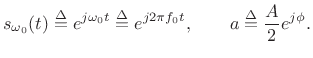
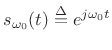
We see that, since the Fourier transform is a linear operator, we need only work with the unit-amplitude, zero-phase, positive-frequency sinusoid
 . For
. For
It remains to find the Fourier transform of
![]() :
:
![\begin{eqnarray*}
S_{\omega_0}(\omega)
&=& \int_{-\infty}^{\infty} s_{\omega_0}(t) e^{-j\omega t} dt\\ [5pt]
&\isdef & \int_{-\infty}^{\infty} e^{j\omega_0 t} e^{-j\omega t} dt\\ [5pt]
&=& \int_{-\infty}^{\infty} e^{j(\omega_0-\omega) t} dt\\ [5pt]
&=& \left.\frac{1}{j(\omega_0-\omega)} e^{j(\omega_0-\omega) t}
\right\vert _{-\infty}^\infty\\ [5pt]
&=& \lim_{\Delta\to\infty} 2\frac{\sin[(\omega_0-\omega)\Delta]}{\omega_0-\omega}\\ [5pt]
&=& 2\pi\delta(\omega_0-\omega) = \delta(f_0-f),
\end{eqnarray*}](http://www.dsprelated.com/josimages_new/sasp2/img902.png)
where
![]() is the delta function or impulse
at frequency
is the delta function or impulse
at frequency ![]() (see Fig.5.4 for a plot, and
§B.10 for a mathematical introduction).
Since the delta function is even (
(see Fig.5.4 for a plot, and
§B.10 for a mathematical introduction).
Since the delta function is even (
![]() ),
we can also write
),
we can also write
![]() . It is shown in §B.13 that the
sinc
limit
above approaches a delta function
. It is shown in §B.13 that the
sinc
limit
above approaches a delta function
![]() .
However, we will only use the Discrete Fourier Transform (DFT)
in any practical applications, and in that case, the result is easy to
show [264].
.
However, we will only use the Discrete Fourier Transform (DFT)
in any practical applications, and in that case, the result is easy to
show [264].
The inverse Fourier transform is easy to evaluate by the sifting property6.3of delta functions:
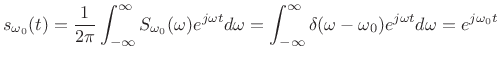 |
(6.6) |
Substituting into (5.4), the spectrum of our original sinusoid
![]() is given by
is given by
| (6.7) |
which is a pair of impulses, one at frequency
Next Section:
Spectrum of Sampled Complex Sinusoid
Previous Section:
Optimal FIR Digital Filter Design


