


WOLA Processing Steps
The sequence of operations in a WOLA processor can be expressed as follows:
- Extract the
 th windowed frame of data
 ,
,
 (assuming a length
  causal window
  and hop
size
and hop
size  ).
).
- Take an FFT of the
th frame translated to time zero,
 , to produce the
th spectral frame
, to produce the
th spectral frame
 ,
,
 .
.
- Process
as desired to produce
 .
.
- Inverse FFT
 to produce
 ,
,
 .
.
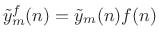
- Apply a synthesis window
 to
to yield a
weighted output frame
to
to yield a
weighted output frame
 ,
.
,
.
- Translate the
th output frame to time
 as
as
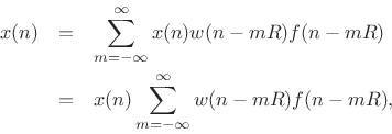
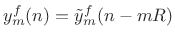 and add to the accumulated output signal
  .
.
To obtain perfect reconstruction in the absence of spectral modifications, we require
which is true if and only if
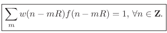 |
(9.44) |
Choice of WOLA Window
The synthesis (output) window in weighted overlap-add is typically chosen to be the same as the analysis (input) window, in which case the COLA constraint becomes
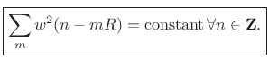 |
(9.45) |
We can say that
A trivial way to construct useful windows for WOLA is to take the
square root of any good OLA window. This works for all non-negative
OLA windows (which covers essentially all windows in Chapter 3
other than Portnoff windows). For example, the
``root-Hann window'' can be defined for odd ![]() by
by
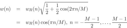
Notice that the root-Hann window is the same thing as the ``MLT Sine Window'' described in §3.2.6. We can similarly define the ``root-Hamming'', ``root-Blackman'', and so on, all of which give perfect reconstruction in the weighted overlap-add context.
Next Section:
Overlap-Add (OLA) Interpretation of the STFT
Previous Section:
Length L FIR Frame Filters


