


Group Delay
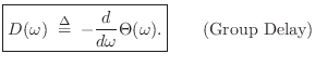
A more commonly encountered representation of filter phase response is called the group delay, defined by
An example of a linear phase response is that of the simplest lowpass
filter,
![]() . Thus, both the phase delay and the group
delay of the simplest lowpass filter are equal to half a sample at
every frequency.
. Thus, both the phase delay and the group
delay of the simplest lowpass filter are equal to half a sample at
every frequency.
For any reasonably smooth phase function, the group delay ![]() may be interpreted as the time delay of the amplitude envelope
of a sinusoid at frequency
may be interpreted as the time delay of the amplitude envelope
of a sinusoid at frequency ![]() [63]. The bandwidth of
the amplitude envelope in this interpretation must be restricted to a
frequency interval over which the phase response is approximately
linear. We derive this result in the next subsection.
[63]. The bandwidth of
the amplitude envelope in this interpretation must be restricted to a
frequency interval over which the phase response is approximately
linear. We derive this result in the next subsection.
Thus, the name ``group delay'' for ![]() refers to the fact that
it specifies the delay experienced by a narrow-band ``group'' of
sinusoidal components which have frequencies within a narrow frequency
interval about
refers to the fact that
it specifies the delay experienced by a narrow-band ``group'' of
sinusoidal components which have frequencies within a narrow frequency
interval about ![]() . The width of this interval is limited to
that over which
. The width of this interval is limited to
that over which ![]() is approximately constant.
is approximately constant.
Derivation of Group Delay as Modulation Delay
Suppose we write a narrowband signal centered at frequency ![]() as
as
where
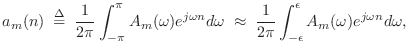
Using the above frequency-domain expansion of ![]() ,
, ![]() can be
written as
can be
written as
![$\displaystyle x(n) \eqsp a_m(n) e^{j\omega_c n} \eqsp
\left[\frac{1}{2\pi} \int_{-\epsilon}^{\epsilon} A_m(\omega)e^{j\omega n} d\omega\right] e^{j\omega_c n},
$](http://www.dsprelated.com/josimages_new/filters/img908.png)
Assuming the phase response
![\begin{eqnarray*}
y_\omega(n)
&=& \left[G(\omega_c+\omega)A_m(\omega)\right]
e^...
...\right]
e^{j\omega[n-D(\omega_c)]} e^{j\omega_c[n-P(\omega_c)]},
\end{eqnarray*}](http://www.dsprelated.com/josimages_new/filters/img916.png)
where we also used the definition of phase delay,
![]() , in the last step. In this expression we
can already see that the carrier sinusoid is delayed by the phase
delay, while the amplitude-envelope frequency-component is delayed by
the group delay. Integrating over
, in the last step. In this expression we
can already see that the carrier sinusoid is delayed by the phase
delay, while the amplitude-envelope frequency-component is delayed by
the group delay. Integrating over ![]() to recombine the
sinusoidal components (i.e., using a Fourier superposition integral for
to recombine the
sinusoidal components (i.e., using a Fourier superposition integral for
![]() ) gives
) gives
![\begin{eqnarray*}
y(n) &=& \frac{1}{2\pi}\int_{\omega} y_\omega(n) d\omega \\
&...
...)]}\\
&=& a^f[n-D(\omega_c)] \cdot e^{j\omega_c[n-P(\omega_c)]}
\end{eqnarray*}](http://www.dsprelated.com/josimages_new/filters/img918.png)
where ![]() denotes a zero-phase filtering of the amplitude
envelope
denotes a zero-phase filtering of the amplitude
envelope ![]() by
by
![]() . We see that the amplitude
modulation is delayed by
. We see that the amplitude
modulation is delayed by
![]() while the carrier wave is
delayed by
while the carrier wave is
delayed by
![]() .
.
We have shown that, for narrowband signals expressed as in
Eq.![]() (7.6) as a modulation envelope times a sinusoidal carrier, the
carrier wave is delayed by the filter phase delay, while the
modulation is delayed by the filter group delay, provided that the
filter phase response is approximately linear over the narrowband
frequency interval.
(7.6) as a modulation envelope times a sinusoidal carrier, the
carrier wave is delayed by the filter phase delay, while the
modulation is delayed by the filter group delay, provided that the
filter phase response is approximately linear over the narrowband
frequency interval.
Next Section:
Group Delay Examples in Matlab
Previous Section:
Phase Unwrapping


