DSPRelated.com
Free Books

Decimation in Time

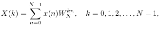
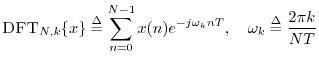
The DFT is defined by
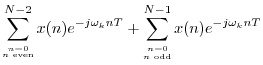
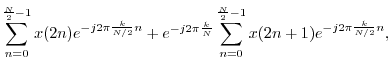
$\displaystyle X(k) = \sum_{n=0}^{N-1} x(n) W_N^{kn}, \quad k=0,1,2,\ldots,N-1,
$

where $ x(n)$ is the input signal amplitude at time $ n$, and

$\displaystyle W_N \isdef e^{-j\frac{2\pi}{N}}.\quad \hbox{(primitive $N$th root of unity)}
$

Note that $ W_N^N=1$.

When $ N$ is even, the DFT summation can be split into sums over the odd and even indexes of the input signal:
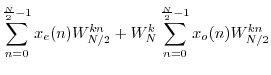
$\displaystyle X(\omega_k)$ $\displaystyle \isdef$ $\displaystyle \hbox{\sc DFT}_{{N,k}}\{x\} \isdef \sum_{n=0}^{N-1} x(n) e^{-j\omega_k n T},
\quad \omega_k \isdef \frac{2\pi k}{NT}$  
  $\displaystyle =$ $\displaystyle \sum_{{\stackrel{n=0}{\vspace{2pt}\mbox{\tiny$n$\ even}}}}^{N-2} ...
...stackrel{n=0}{\vspace{2pt}\mbox{\tiny$n$\ odd}}}}^{N-1} x(n) e^{-j\omega_k n T}$  
  $\displaystyle =$ $\displaystyle \sum_{n=0}^{\frac{N}{2}-1} x(2n) e^{-j2\pi \frac{k}{N/2} n}
+ e^{-j2\pi\frac{k}{N}}\sum_{n=0}^{\frac{N}{2}-1} x(2n+1) e^{-j2\pi \frac{k}{N/2} n},$  
  $\displaystyle =$ $\displaystyle \sum_{n=0}^{\frac{N}{2}-1} x_e(n) W_{N/2}^{kn} + W_N^k
\sum_{n=0}^{\frac{N}{2}-1} x_o(n) W_{N/2}^{kn}$  
  $\displaystyle \isdef$ $\displaystyle \hbox{\sc DFT}_{{\frac{N}{2},k}}\{\hbox{\sc Downsample}_2(x)\}$  
    $\displaystyle \mathop{\quad} +\;W_N^k\cdot\hbox{\sc DFT}_{{\frac{N}{2},k}}\{\hbox{\sc Downsample}_2[\hbox{\sc Shift}_1(x)]\},
\protect$ (A.1)

where $ x_e(n)\isdef x(2n)$ and $ x_o(n)\isdef x(2n+1)$ denote the even- and odd-indexed samples from $ x$. Thus, the length $ N$ DFT is computable using two length $ N/2$ DFTs. The complex factors $ W_N^k=e^{-j\omega_k}=\exp(-j2\pi k/N)$ are called twiddle factors. The splitting into sums over even and odd time indexes is called decimation in time. (For decimation in frequency, the inverse DFT of the spectrum $ X(\omega_k)$ is split into sums over even and odd bin numbers $ k$.)


Next Section:
Radix 2 FFT
Previous Section:
Coherence Function in Matlab