


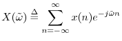
Fourier Transforms for Continuous/Discrete Time/Frequency
The Fourier transform can be defined for signals which are
- discrete or continuous in time, and
- finite or infinite in duration.
- discrete or continuous in frequency, and
- finite or infinite in bandwidth.
This book has been concerned almost exclusively with the discrete-time, discrete-frequency case (the DFT), and in that case, both the time and frequency axes are finite in length. In the following sections, we briefly summarize the other three cases. Table B.1 summarizes all four Fourier-transform cases corresponding to discrete or continuous time and/or frequency.

Discrete Time Fourier Transform (DTFT)
The Discrete Time Fourier Transform (DTFT) can be viewed as the
limiting form of the DFT when its length ![]() is allowed to approach
infinity:
is allowed to approach
infinity:
The inverse DTFT is

Instead of operating on sampled signals of length ![]() (like the DFT),
the DTFT operates on sampled signals
(like the DFT),
the DTFT operates on sampled signals ![]() defined over all integers
defined over all integers
![]() . As a result, the DTFT frequencies form a
continuum. That is, the DTFT is a function of
continuous frequency
. As a result, the DTFT frequencies form a
continuum. That is, the DTFT is a function of
continuous frequency
![]() , while the DFT is a
function of discrete frequency
, while the DFT is a
function of discrete frequency ![]() ,
,
![]() . The DFT
frequencies
. The DFT
frequencies
![]() ,
,
![]() , are given by
the angles of
, are given by
the angles of ![]() points uniformly distributed along the unit circle
in the complex plane (see
Fig.6.1). Thus, as
points uniformly distributed along the unit circle
in the complex plane (see
Fig.6.1). Thus, as
![]() , a continuous frequency axis
must result in the limit along the unit circle in the
, a continuous frequency axis
must result in the limit along the unit circle in the ![]() plane. The
axis is still finite in length, however, because the time domain
remains sampled.
plane. The
axis is still finite in length, however, because the time domain
remains sampled.
Fourier Transform (FT) and Inverse
The Fourier transform of a signal
![]() ,
,
![]() , is defined as
, is defined as
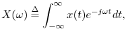
and its inverse is given by

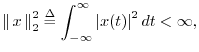
Existence of the Fourier Transform
Conditions for the existence of the Fourier transform are
complicated to state in general [12], but it is sufficient
for ![]() to be absolutely integrable, i.e.,
to be absolutely integrable, i.e.,

There is never a question of existence, of course, for Fourier transforms of real-world signals encountered in practice. However, idealized signals, such as sinusoids that go on forever in time, do pose normalization difficulties. In practical engineering analysis, these difficulties are resolved using Dirac's ``generalized functions'' such as the impulse (also called the delta function) [38].
The Continuous-Time Impulse
An impulse in continuous time must have ``zero width'' and unit area under it. One definition is
![$\displaystyle \delta(t) \isdef \lim_{\Delta \to 0} \left\{\begin{array}{ll} \fr...
...eq t\leq \Delta \\ [5pt] 0, & \hbox{otherwise}. \\ \end{array} \right. \protect$](http://www.dsprelated.com/josimages_new/mdft/img1700.png)
An impulse can be similarly defined as the limit of any integrable pulse shape which maintains unit area and approaches zero width at time 0. As a result, the impulse under every definition has the so-called sifting property under integration,
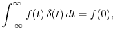
provided
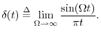
An impulse is not a function in the usual sense, so it is called instead a distribution or generalized function [12,38]. (It is still commonly called a ``delta function'', however, despite the misnomer.)
Fourier Series (FS) and Relation to DFT
In continuous time, a periodic signal ![]() , with period
, with period ![]() seconds,B.2 may be expanded
into a Fourier series with coefficients given by
seconds,B.2 may be expanded
into a Fourier series with coefficients given by
where
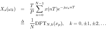
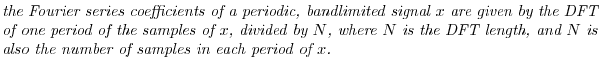
Relation of the DFT to Fourier Series
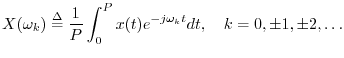
We now show that the DFT of a sampled signal ![]() (of length
(of length ![]() ),
is proportional to the
Fourier series coefficients of the continuous
periodic signal obtained by
repeating and interpolating
),
is proportional to the
Fourier series coefficients of the continuous
periodic signal obtained by
repeating and interpolating ![]() . More precisely, the DFT of the
. More precisely, the DFT of the ![]() samples comprising one period equals
samples comprising one period equals ![]() times the Fourier series
coefficients. To avoid aliasing upon sampling, the continuous-time
signal must be bandlimited to less than half the sampling
rate (see Appendix D); this implies that at most
times the Fourier series
coefficients. To avoid aliasing upon sampling, the continuous-time
signal must be bandlimited to less than half the sampling
rate (see Appendix D); this implies that at most ![]() complex harmonic components can be nonzero in the original
continuous-time signal.
complex harmonic components can be nonzero in the original
continuous-time signal.
If ![]() is bandlimited to
is bandlimited to
![]() , it can be sampled
at intervals of
, it can be sampled
at intervals of ![]() seconds without aliasing (see
§D.2). One way to sample a signal inside an integral
expression such as
Eq.
seconds without aliasing (see
§D.2). One way to sample a signal inside an integral
expression such as
Eq.![]() (B.5) is to multiply it by a continuous-time impulse train
(B.5) is to multiply it by a continuous-time impulse train
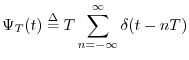
where
We wish to find the continuous-time Fourier series of the
sampled periodic signal ![]() . Thus, we replace
. Thus, we replace ![]() in
Eq.
in
Eq.![]() (B.5) by
(B.5) by
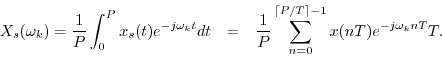
If the sampling interval ![]() is chosen so that it divides the signal
period
is chosen so that it divides the signal
period ![]() , then the number of samples under the integral is an integer
, then the number of samples under the integral is an integer
![]() , and we obtain
, and we obtain
where
![]() . Thus,
. Thus,
![]() for all
for all ![]() at which the bandlimited
periodic signal
at which the bandlimited
periodic signal ![]() has a nonzero harmonic. When
has a nonzero harmonic. When ![]() is odd,
is odd,
![]() can be nonzero for
can be nonzero for
![]() , while for
, while for
![]() even, the maximum nonzero harmonic-number range is
even, the maximum nonzero harmonic-number range is
![]() .
.
In summary,
Next Section:
Selected Continuous-Time Fourier Theorems
Previous Section:
Fast Fourier Transform (FFT) Algorithms


