


Matlab/Octave Examples
This appendix provides Matlab and Octave examples for various topics covered in this book. The term `matlab' (uncapitalized) refers to either Matlab or Octave [67].
Complex Numbers in Matlab and Octave
Matlab and Octave have the following primitives for complex numbers:
octave:1> help j

j is a built-in constant

 - Built-in Variable: I
 - Built-in Variable: J
 - Built-in Variable: i
 - Built-in Variable: j

A pure imaginary number, defined as `sqrt (-1)'.  The `I' and `J'
forms are true constants, and cannot be modified.  The `i' and `j'
forms are like ordinary variables, and may be used for other
purposes.  However, unlike other variables, they once again assume
their special predefined values if they are cleared *Note Status
of Variables::.

Additional help for built-in functions, operators, and variables
is available in the on-line version of the manual.  Use the command
`help -i <topic>' to search the manual index.

Help and information about Octave is also available on the WWW
at http://www.octave.org and via the help-octave@bevo.che.wisc.edu
mailing list.

octave:2> sqrt(-1)
ans = 0 + 1i

octave:3> help real
real is a built-in mapper function

 - Mapping Function:  real (Z)
     Return the real part of Z.

See also: imag and conj. ...

octave:4> help imag
imag is a built-in mapper function

 - Mapping Function:  imag (Z)
     Return the imaginary part of Z as a real number.

See also: real and conj. ...

octave:5> help conj
conj is a built-in mapper function

 - Mapping Function:  conj (Z)
     Return the complex conjugate of Z, defined as
     `conj (Z)' = X - IY.

See also: real and imag. ...

octave:6> help abs
abs is a built-in mapper function

 - Mapping Function:  abs (Z)
     Compute the magnitude of Z, defined as
     |Z| = `sqrt (x^2 + y^2)'.

     For example,

          abs (3 + 4i)
          => 5
...
octave:7> help angle
angle is a built-in mapper function

 - Mapping Function:  angle (Z)
     See arg.
...
Note how helpful the ``See also'' information is in Octave (and
similarly in Matlab).
Complex Number Manipulation
Let's run through a few elementary manipulations of complex numbers in Matlab:
>> x = 1;
>> y = 2;
>> z = x + j * y

z =
   1 + 2i

>> 1/z

ans =
   0.2 - 0.4i

>> z^2

ans =
  -3 + 4i

>> conj(z)

ans =
   1 - 2i

>> z*conj(z)

ans =
     5

>> abs(z)^2

ans =
    5

>> norm(z)^2

ans =
    5

>> angle(z)

ans =
    1.1071
Now let's do polar form:
>> r = abs(z)

r =
    2.2361

>> theta = angle(z)

theta =
    1.1071
Curiously, ![]() is not defined by default in Matlab (though it is in
Octave). It can easily be computed in Matlab as
is not defined by default in Matlab (though it is in
Octave). It can easily be computed in Matlab as e=exp(1).
Below are some examples involving imaginary exponentials:
>> r * exp(j * theta)

ans =
   1 + 2i

>> z

z =
   1 + 2i

>> z/abs(z)

ans =
   0.4472 + 0.8944i

>> exp(j*theta)

ans =
   0.4472 + 0.8944i

>> z/conj(z)

ans =
  -0.6 + 0.8i

>> exp(2*j*theta)

ans =
  -0.6 + 0.8i

>> imag(log(z/abs(z)))

ans =
    1.1071

>> theta

theta =
    1.1071

>>
Here are some manipulations involving two complex numbers:
>> x1 = 1;
>> x2 = 2;
>> y1 = 3;
>> y2 = 4;
>> z1 = x1 + j * y1;
>> z2 = x2 + j * y2;
>> z1

z1 =
   1 + 3i

>> z2

z2 =
   2 + 4i

>> z1*z2

ans =
 -10 +10i

>> z1/z2

ans =
   0.7 + 0.1i
Another thing to note about matlab syntax is that the transpose operator ' (for vectors and matrices) conjugates as well as transposes. Use .' to transpose without conjugation:
>>x = [1:4]*j

x =
        0 + 1i   0 + 2i   0 + 3i   0 + 4i

>> x'

ans =
        0 - 1i
        0 - 2i
        0 - 3i
        0 - 4i

>> x.'

ans =
        0 + 1i
        0 + 2i
        0 + 3i
        0 + 4i
Factoring Polynomials in Matlab
Let's find all roots of the polynomial
>> % polynomial = array of coefficients in matlab:
>> p = [1 0 0 0 5 7]; %  p(x) = x^5 + 5*x + 7
>> format long;       %  print double-precision
>> roots(p)           %  print out the roots of p(x)

ans =
  1.30051917307206 + 1.10944723819596i
  1.30051917307206 - 1.10944723819596i
 -0.75504792501755 + 1.27501061923774i
 -0.75504792501755 - 1.27501061923774i
 -1.09094249610903
Geometric Signal Theory
This section follows Chapter 5 of the text.
Vector Interpretation of Complex Numbers
Here's how Fig.5.1 may be generated in matlab:
>> x = [2 3];                  % coordinates of x
>> origin = [0 0];             % coordinates of the origin
>> xcoords = [origin(1) x(1)]; % plot() expects coordinates
>> ycoords = [origin(2) x(2)];
>> plot(xcoords,ycoords);      % Draw a line from origin to x
Signal Metrics
The mean of a signal ![]() stored in a matlab row- or column-vector
x can be computed in matlab as
stored in a matlab row- or column-vector
x can be computed in matlab as
mu = sum(x)/Nor by using the built-in function mean(). If x is a 2D matrix containing N elements, then we need mu = sum(sum(x))/N or mu = mean(mean(x)), since sum computes a sum along ``dimension 1'' (which is along columns for matrices), and mean is implemented in terms of sum. For 3D matrices, mu = mean(mean(mean(x))), etc. For a higher dimensional matrices x, ``flattening'' it into a long column-vector x(:) is the more concise form:
N = prod(size(x))
mu = sum(x(:))/N
or
mu = x(:).' * ones(N,1)/NThe above constructs work whether x is a row-vector, column-vector, or matrix, because x(:) returns a concatenation of all columns of x into one long column-vector. Note the use of .' to obtain non-conjugating vector transposition in the second form. N = prod(size(x)) is the number of elements of x. If x is a row- or column-vector, then length(x) gives the number of elements. For matrices, length() returns the greater of the number of rows or columns.I.1
Signal Energy and Power
In a similar way, we can compute the signal energy
![]() (sum of squared moduli) using any of the following constructs:
(sum of squared moduli) using any of the following constructs:
Ex = x(:)' * x(:)
Ex = sum(conj(x(:)) .* x(:))
Ex = sum(abs(x(:)).^2)
The average power (energy per sample) is similarly Px = Ex/N. The
Inner Product
The inner product
![]() of two column-vectors x and
y (§5.9)
is conveniently computed in matlab as
of two column-vectors x and
y (§5.9)
is conveniently computed in matlab as
xdoty = y' * x
Vector Cosine
For real vectors x and y having the same length, we may compute the vector cosine by
cosxy = y' * x / ( norm(x) * norm(y) );For complex vectors, a good measure of orthogonality is the modulus of the vector cosine:
collinearity = abs(y' * x) / ( norm(x) * norm(y) );Thus, when collinearity is near 0, the vectors x and y are substantially orthogonal. When collinearity is close to 1, they are nearly collinear.
Projection
As discussed in §5.9.9,
the orthogonal projection of
![]() onto
onto
![]() is defined by
is defined by
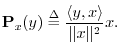
yx = (x' * y) * (x' * x)^(-1) * xMore generally, a length-N column-vector y can be projected onto the
yX = X * (X' * X)^(-1) * X' * yOrthogonal projection, like any finite-dimensional linear operator, can be represented by a matrix. In this case, the
PX = X * (X' * X)^(-1) * X'is called the projection matrix.I.2Subspace projection is an example in which the power of matrix linear algebra notation is evident.
Projection Example 1
>> X = [[1;2;3],[1;0;1]]
X =

   1   1
   2   0
   3   1

>> PX = X * (X' * X)^(-1) * X'
PX =

   0.66667  -0.33333   0.33333
  -0.33333   0.66667   0.33333
   0.33333   0.33333   0.66667

>> y = [2;4;6]
y =

   2
   4
   6

>> yX = PX * y
yX =

   2.0000
   4.0000
   6.0000
Since y in this example already lies in the column-space of X, orthogonal projection onto that space has no effect.
Projection Example 2
Let X and PX be defined as Example 1, but now let
>> y = [1;-1;1]
y =

   1
  -1
   1

>> yX = PX * y
yX =

   1.33333
  -0.66667
   0.66667

>> yX' * (y-yX)
ans = -7.0316e-16

>> eps
ans =  2.2204e-16
In the last step above, we verified that the projection yX is
orthogonal to the ``projection error'' y-yX, at least to
machine precision. The eps variable holds ``machine
epsilon'' which is the numerical distance
between ![]() and the next representable number in double-precision
floating point.
and the next representable number in double-precision
floating point.
Orthogonal Basis Computation
Matlab and Octave have a function orth() which will compute an orthonormal basis for a space given any set of vectors which span the space. In Matlab, e.g., we have the following help info:
>> help orth
 ORTH  Orthogonalization.
       Q = orth(A) is an orthonormal basis for the range of A.
       Q'*Q = I, the columns of Q span the same space as the
       columns of A and the number of columns of Q is the rank
       of A.

       See also QR, NULL.
Below is an example of using orth() to orthonormalize a linearly
independent basis set for ![]() :
:
% Demonstration of the orth() function.
v1 = [1; 2; 3];  % our first basis vector (a column vector)
v2 = [1; -2; 3]; % a second, linearly independent vector
v1' * v2         % show that v1 is not orthogonal to v2

ans =
     6

V = [v1,v2]      % Each column of V is one of our vectors

V =
     1     1
     2    -2
     3     3

W = orth(V)  % Find an orthonormal basis for the same space

W =
    0.2673    0.1690
    0.5345   -0.8452
    0.8018    0.5071

w1 = W(:,1)  % Break out the returned vectors

w1 =
    0.2673
    0.5345
    0.8018

w2 = W(:,2)

w2 =
    0.1690
   -0.8452
    0.5071

w1' * w2  % Check that w1 is orthogonal to w2

ans =
   2.5723e-17

w1' * w1  % Also check that the new vectors are unit length

ans =
     1

w2' * w2

ans =
     1

W' * W   % faster way to do the above checks

ans =
    1    0
    0    1


% Construct some vector x in the space spanned by v1 and v2:
x = 2 * v1 - 3 * v2

x =
    -1
    10
    -3

% Show that x is also some linear combination of w1 and w2:
c1 = x' * w1      % Coefficient of projection of x onto w1

c1 =
    2.6726

c2 = x' * w2      % Coefficient of projection of x onto w2

c2 =
  -10.1419

xw = c1 * w1 + c2 * w2  % Can we make x using w1 and w2?

xw =
   -1
   10
   -3

error = x - xw

error = 1.0e-14 *

    0.1332
         0
         0

norm(error)       % typical way to summarize a vector error

ans =
   1.3323e-15

% It works! (to working precision, of course)
% Construct a vector x NOT in the space spanned by v1 and v2:
y = [1; 0; 0];     % Almost anything we guess in 3D will work

%  Try to express y as a linear combination of w1 and w2:
c1 = y' * w1;      % Coefficient of projection of y onto w1
c2 = y' * w2;      % Coefficient of projection of y onto w2
yw = c1 * w1 + c2 * w2  % Can we make y using w1 and w2?
yw =

    0.1
    0.0
    0.3

yerror = y - yw

yerror =

    0.9
    0.0
   -0.3

norm(yerror)

ans =
    0.9487
While the error is not zero, it is the smallest possible error in the
least squares sense. That is, yw is the optimal
least-squares approximation to y in the space spanned by v1
and v2 (w1 and w2). In other words,
norm(yerror) is less than or equal to norm(y-yw2) for any
other vector yw2 made using a linear combination of
v1 and v2. In yet other words, we obtain the
optimal least squares approximation of
y (which lives in 3D) in some subspace ![]() (a 2D subspace of 3D
spanned by the columns of matrix W) by projecting
y orthogonally onto the subspace
(a 2D subspace of 3D
spanned by the columns of matrix W) by projecting
y orthogonally onto the subspace ![]() to get
yw as above.
to get
yw as above.
An important property of the optimal least-squares approximation is that the approximation error is orthogonal to the the subspace in which the approximation lies. Let's verify this:
W' * yerror   % must be zero to working precision

ans = 1.0e-16 *

   -0.2574
   -0.0119
The DFT
This section gives Matlab examples illustrating the computation of two figures in Chapter 6, and the DFT matrix in Matlab.
DFT Sinusoids for 
Below is the Matlab for Fig.6.2:
N=8;
fs=1;

n = [0:N-1]; % row
t = [0:0.01:N]; % interpolated
k=fliplr(n)' - N/2;
fk = k*fs/N;
wk = 2*pi*fk;
clf;
for i=1:N
  subplot(N,2,2*i-1);
  plot(t,cos(wk(i)*t))
  axis([0,8,-1,1]);
  hold on;
  plot(n,cos(wk(i)*n),'*')
  if i==1
    title('Real Part');
  end;
  ylabel(sprintf('k=%d',k(i)));
  if i==N
    xlabel('Time (samples)');
  end;
  subplot(N,2,2*i);
  plot(t,sin(wk(i)*t))
  axis([0,8,-1,1]);
  hold on;
  plot(n,sin(wk(i)*n),'*')
  ylabel(sprintf('k=%d',k(i)));
  if i==1
    title('Imaginary Part');
  end;
  if i==N
    xlabel('Time (samples)');
  end;
end
DFT Bin Response
Below is the Matlab for Fig.6.3:
% Parameters (sampling rate = 1)
N = 16;               % DFT length
k = N/4;              % bin where DFT filter is centered
wk = 2*pi*k/N;        % normalized radian center-frequency
wStep = 2*pi/N;
w = [0:wStep:2*pi - wStep]; % DFT frequency grid

interp = 10;
N2 = interp*N; % Denser grid showing "arbitrary" frequencies
w2Step = 2*pi/N2;
w2 = [0:w2Step:2*pi - w2Step]; % Extra dense frequency grid
X = (1 - exp(j*(w2-wk)*N)) ./ (1 - exp(j*(w2-wk)));
X(1+k*interp) = N; % Fix divide-by-zero point (overwrite NaN)

% Plot spectral magnitude
clf;
magX = abs(X);
magXd = magX(1:interp:N2); % DFT frequencies only
subplot(2,1,1);
plot(w2,magX,'-'); hold on; grid;
plot(w,magXd,'*');         % Show DFT sample points
title('DFT Amplitude Response at k=N/4');
xlabel('Normalized Radian Frequency (radians per sample)');
ylabel('Magnitude (Linear)');
text(-1,20,'a)');

% Same thing on a dB scale
magXdb = 20*log10(magX);       % Spectral magnitude in dB
% Since the zeros go to minus infinity, clip at -60 dB:
magXdb = max(magXdb,-60*ones(1,N2));
magXddb = magXdb(1:interp:N2); % DFT frequencies only
subplot(2,1,2);
hold off; plot(w2,magXdb,'-'); hold on; plot(w,magXddb,'*');
xlabel('Normalized Radian Frequency (radians per sample)');
ylabel('Magnitude (dB)'); grid;
text(-1,40,'b)');
print -deps '../eps/dftfilter.eps';
hold off;
DFT Matrix
The following example reinforces the discussion of the DFT matrix in §6.12. We can simply create the DFT matrix in matlab by taking the DFT of the identity matrix. Then we show that multiplying by the DFT matrix is equivalent to the calling the fft function in matlab:
>> eye(4)
ans =
     1     0     0     0
     0     1     0     0
     0     0     1     0
     0     0     0     1

>> S4 = fft(eye(4))
ans =
   1       1          1       1
   1       0 - 1i    -1       0 + 1i
   1      -1          1      -1
   1       0 + 1i    -1       0 - 1i

>> S4' * S4          % Show that S4' = inverse DFT (times N=4)
ans =
    4    0    0    0
    0    4    0    0
    0    0    4    0
    0    0    0    4

>> x = [1; 2; 3; 4]
x =
     1
     2
     3
     4
>> fft(x)
ans =
  10
  -2 + 2i
  -2
  -2 - 2i

>> S4 * x
ans =
  10
  -2 + 2i
  -2
  -2 - 2i
Spectrogram Computation
This section lists the spectrogram function called in the Matlab code displayed in Fig.8.11.
function X = spectrogram(x,nfft,fs,window,noverlap,doplot,dbclip);

%SPECTROGRAM Calculate spectrogram from signal.
% B = SPECTROGRAM(A,NFFT,Fs,WINDOW,NOVERLAP) calculates the
%     spectrogram for the signal in vector A.
%
% NFFT is the FFT size used for each frame of A.  It should be a
% power of 2 for fastest computation of the spectrogram.
%
% Fs is the sampling frequency. Since all processing parameters are
% in units of samples, Fs does not effect the spectrogram itself,
% but it is used for axis scaling in the plot produced when
% SPECTROGRAM is called with no output argument (see below).
%
% WINDOW is the length M window function applied, IN ZERO-PHASE
% FORM, to each frame of A.  M cannot exceed NFFT.  For M<NFFT,
% NFFT-M zeros are inserted in the FFT buffer (for interpolated
% zero-phase processing).  The window should be supplied in CAUSAL
% FORM.
%
% NOVERLAP is the number of samples the sections of A overlap, if
% nonnegative.  If negative, -NOVERLAP is the "hop size", i.e., the
% number of samples to advance successive windows.  (The overlap is
% the window length minus the hop size.)  The hop size is called
% NHOP below.  NOVERLAP must be less than M.
%
% If doplot is nonzero, or if there is no output argument, the
% spectrogram is displayed.
%
% When the spectrogram is displayed, it is "clipped" dbclip dB
% below its maximum magnitude.  The default clipping level is 100
% dB down.
%
% Thus, SPECTROGRAM splits the signal into overlapping segments of
% length M, windows each segment with the length M WINDOW vector, in
% zero-phase form, and forms the columns of B with their
% zero-padded, length NFFT discrete Fourier transforms.
%
% With no output argument B, SPECTROGRAM plots the dB magnitude of
% the spectrogram in the current figure, using
% IMAGESC(T,F,20*log10(ABS(B))), AXIS XY, COLORMAP(JET) so the low
% frequency content of the first portion of the signal is displayed
% in the lower left corner of the axes.
%
% Each column of B contains an estimate of the short-term,
% time-localized frequency content of the signal A.  Time increases
% linearly across the columns of B, from left to right.  Frequency
% increases linearly down the rows, starting at 0.
%
% If A is a length NX complex signal, B is returned as a complex
% matrix with NFFT rows and
%      k = floor((NX-NOVERLAP)/(length(WINDOW)-NOVERLAP))
%        = floor((NX-NOVERLAP)/NHOP)
% columns.  When A is real, only the NFFT/2+1 rows are needed when
% NFFT even, and the first (NFFT+1)/2 rows are sufficient for
% inversion when NFFT is odd.
%
% See also: Matlab and Octave's SPECGRAM and STFT functions.

if nargin<7, dbclip=100; end
if nargin<6, doplot=0; end
if nargin<5, noverlap=256; end
if nargin<4, window=hamming(512); end
if nargin<3, fs=1; end
if nargin<2, nfft=2048; end

x = x(:); % make sure it's a column

M = length(window);
if length(x)<M, x = [x;zeros(M-length(x),1)]; end;
if (M<2)
  % (Matlab's specgram allows window to be a scalar specifying
  % the length of a Hanning window.)
  error('spectrogram: Expect complete window, not just its length');
end;
Modd = mod(M,2); % 0 if M even, 1 if odd
Mo2 = (M-Modd)/2;
w = window(:); % Make sure it's a column
zp = zeros(nfft-M,1);
wzp = [w(Mo2+1:M);zp;w(1:Mo2)];

noverlap = round(noverlap); % in case non-integer
if noverlap<0
  nhop = - noverlap;
  noverlap = M-nhop;
else
  nhop = M-noverlap;
end

nx = length(x);
nframes = 1+floor((nx-noverlap)/nhop);

X = zeros(nfft,nframes);
xoff = 0;
for m=1:nframes-1
  xframe = x(xoff+1:xoff+M); % extract frame of input data
  xoff = xoff + nhop;   % advance in-pointer by hop size
  xzp = [xframe(Mo2+1:M);zp;xframe(1:Mo2)];
  xw = wzp .* xzp;
  X(:,m) = fft(xw);
end

if (nargout==0) | doplot
  t = (0:nframes-1)*nhop/fs;
  f = 0.001*(0:nfft-1)*fs/nfft;
  Xdb = 20*log10(abs(X));
  Xmax = max(max(Xdb));
  % Clip lower limit so nulls don't dominate:
  clipvals = [Xmax-dbclip,Xmax];
  imagesc(t,f,Xdb,clipvals);
  % grid;
  axis('xy');
  colormap(jet);
  xlabel('Time (sec)');
  ylabel('Freq (kHz)');
end
Bibliography
- 1
- M. Abramowitz and I. A. Stegun, eds., Handbook of Mathematical Functions,
New York: Dover, 1965.- 2
- R. Agarwal and C. S. Burrus, ``Number theoretic transforms to implement fast digital convolution,'' Proceedings of the IEEE, vol. 63, pp. 550-560, Apr. 1975,
also in [43].- 3
- J. B. Allen and L. R. Rabiner, ``A unified approach to short-time Fourier analysis and synthesis,'' Proc. IEEE, vol. 65, pp. 1558-1564, Nov. 1977.
- 4
- L. Beranek, Concert Halls and Opera Houses: Music, Acoustics, and Architecture,
Berlin: Springer-Verlag, 2004.- 5
- M. Bosi and R. E. Goldberg, Introduction to Digital Audio Coding and Standards,
Boston: Kluwer Academic Publishers, 2003.- 6
- L. Bosse, ``An experimental high fidelity perceptual audio coder,'' tech. rep., Elec. Engineering Dept., Stanford University (CCRMA), Mar. 1998,
Music 420 Project Report, http://ccrma.stanford.edu/~jos/bosse/.- 7
- K. Brandenburg and M. Bosi, ``Overview of MPEG audio: Current and future standards for low-bit-rate audio coding,'' Journal of the Audio Engineering Society, vol. 45, pp. 4-21, Jan./Feb. 1997.
- 8
- R. Bristow-Johnson, ``Tutorial on floating-point versus fixed-point,'' Audio Engineering Society Convention, Oct. 2008.
- 9
- C. S. Burrus, ``Notes on the FFT,'' Mar. 1990.
- 10
- C. S. Burrus and T. W. Parks, DFT/FFT and Convolution Algorithms,
New York: John Wiley and Sons, Inc., 1985.- 11
- J. P. Campbell Jr., T. E. Tremain, and V. C. Welch, ``The proposed federal standard 1016 4800 bps voice coder: CELP,'' Speech Technology Magazine, pp. 58-64, April-May 1990.
- 12
- D. C. Champeney, A Handbook of Fourier Theorems,
Cambridge University Press, 1987.- 13
- D. G. Childers, ed., Modern Spectrum Analysis,
New York: IEEE Press, 1978.- 14
- J. M. Chowning, ``The synthesis of complex audio spectra by means of frequency modulation,'' Journal of the Audio Engineering Society, vol. 21, no. 7, pp. 526-534, 1973,
reprinted in [62].- 15
- R. V. Churchill, Complex Variables and Applications,
New York: McGraw-Hill, 1960.- 16
- J. Cooley and J. Tukey, ``An algorithm for the machine computation of the complex Fourier series,'' Mathematics of Computation, vol. 19, pp. 297-301, Apr. 1965.
- 17
- J. Dattorro, ``The implementation of recursive digital filters for high-fidelity audio,'' Journal of the Audio Engineering Society, vol. 36, pp. 851-878, Nov. 1988,
Comments, ibid. (Letters to the Editor), vol. 37, p. 486 (1989 June); Comments, ibid. (Letters to the Editor), vol. 38, pp. 149-151 (1990 Mar.).- 18
- J. R. Deller Jr., J. G. Proakis, and J. H. Hansen, Discrete-Time Processing of Speech Signals,
New York: Macmillan, 1993.- 19
- P. A. M. Dirac, The Principles of Quantum Mechanics, Fourth Edition,
New York: Oxford University Press, 1958-2001.- 20
- DSP Committee, ed., Programs for Digital Signal Processing,
New York: IEEE Press, 1979.- 21
- P. Duhamel and M. Vetterli, ``Improved Fourier and Hartley algorithms with application to cyclic convolution of real data,'' IEEE Transactions on Acoustics, Speech, Signal Processing, vol. 35, pp. 818-824, June 1987.
- 22
- P. Duhamel and M. Vetterli, ``Fast Fourier transforms: A tutorial review and state of the art,'' Signal Processing, vol. 19, pp. 259-299, Apr. 1990.
- 23
- M. Frigo and S. G. Johnson, ``FFTW: An adaptive software architecture for the FFT,'' in Proceedings of the International Conference on Acoustics, Speech, and Signal Processing, Seattle, vol. 3, (New York), pp. 1381-1384, IEEE Press, 1998,
http://www.fftw.org/.- 24
- B. Gold and C. M. Rader, Digital Processing of Signals,
New York: McGraw-Hill, 1969.- 25
- G. H. Golub and C. F. Van Loan, Matrix Computations, 2nd Edition,
Baltimore: The Johns Hopkins University Press, 1989.- 26
- I. J. Good, ``The interaction algorithm and practical Fourier analysis,'' Journal of the Royal Statistical Society, Series B, vol. 20, no. 2, pp. 361-372, 1958,
addendum: ibid. 22 (2), 373-375 (1960).- 27
- R. M. Gray and L. D. Davisson, An Introduction to Statistical Signal Processing,
Cambridge University Press, 2003,
http://www-ee.stanford.edu/~gray/sp.pdf.- 28
- J. Gullberg, Mathematics From the Birth of Numbers,
New York: Norton and Co., 1997,
[Qa21.G78 1996] ISBN 0-393-04002-X.- 29
- W. Hartmann, Signals, Sound, and Sensation,
New York: AIP Press, 1997,
647 pp., 221 illustrations, hardcover.- 30
- M. Heideman, D. Johnson, and C. S. Burrus, ``Gauss and the history of the FFT,'' IEEE Signal Processing Magazine, vol. 1, pp. 14-21, Oct. 1984,
also in the Archive for History of Exact Sciences, vol. 34, no. 3, pp. 265-277, 1985.- 31
- S. G. Johnson and M. Frigo, ``A modified split-radix FFT with fewer arithmetic operations,'' IEEE Transactions on Signal Processing, vol. 55, pp. 111-119, Jan. 2007.
- 32
- T. Kailath, A. H. Sayed, and B. Hassibi, Linear Estimation,
Englewood Cliffs, NJ: Prentice-Hall, Apr. 2000.- 33
- S. M. Kay, Fundamentals of Statistical Signal Processing, Volume I: Estimation Theory,
Englewood Cliffs, NJ: Prentice-Hall, 1993.- 34
- S. M. Kay, Fundamentals of Statistical Signal Processing, Volume II: Detection Theory,
Englewood Cliffs, NJ: Prentice-Hall, 1998.- 35
- D. Kolba and T. Parks, ``A prime factor FFT algorithm using high-speed convolution,'' IEEE Transactions on Acoustics, Speech, Signal Processing, vol. 29, pp. 281-294, Aug. 1977,
also in [43].- 36
- T. I. Laakso, V. Välimäki, M. Karjalainen, and U. K. Laine, ``Splitting the Unit Delay--Tools for Fractional Delay Filter Design,'' IEEE Signal Processing Magazine, vol. 13, pp. 30-60, Jan. 1996.
- 37
- W. R. LePage, Complex Variables and the Laplace Transform for Engineers,
New York: Dover, 1961.- 38
- M. J. Lighthill, Introduction to Fourier Analysis,
Cambridge University Press, Jan. 1958.- 39
- L. Ljung and T. L. Soderstrom, Theory and Practice of Recursive Identification,
Cambridge, MA: MIT Press, 1983.- 40
- J. Makhoul, ``Linear prediction: A tutorial review,'' Proceedings of the IEEE, vol. 63, pp. 561-580, Apr. 1975.
- 41
- J. D. Markel and A. H. Gray, Linear Prediction of Speech,
New York: Springer Verlag, 1976.- 42
- M. V. Mathews, The Technology of Computer Music,
Cambridge, MA: MIT Press, 1969.- 43
- J. H. McClellan and C. M. Rader, Number Theory in Digital Signal Processing,
Englewood Cliffs, NJ: Prentice-Hall, 1979.- 44
- J. H. McClellan, R. W. Schafer, and M. A. Yoder, DSP First: A Multimedia Approach,
Englewood Cliffs, NJ: Prentice-Hall, 1998,
Tk5102.M388.- 45
- B. C. J. Moore, An Introduction to the Psychology of Hearing,
New York: Academic Press, 1997.- 46
- M. S. Moslehian, T. Rowland, and E. W. Weisstein, Projection Matrix,
From MathWorld-A Wolfram Web Resource, Dec. 2006,
http://mathworld.wolfram.com/ProjectionMatrix.html.- 47
- B. Noble, Applied Linear Algebra,
Englewood Cliffs, NJ: Prentice-Hall, 1969.- 48
- A. V. Oppenheim and R. W. Schafer, Digital Signal Processing,
Englewood Cliffs, NJ: Prentice-Hall, 1975.- 49
- D. O'Shaughnessy, Speech Communication,
Reading MA: Addison-Wesley, 1987.- 50
- T. Painter and A. Spanias, ``Perceptual coding of digital audio,'' Proceedings of the IEEE, vol. 88, pp. 451-513, Apr. 2000.
- 51
- A. Papoulis, Probability, Random Variables, and Stochastic Processes,
New York: McGraw-Hill, 1965.- 52
- A. Papoulis, Signal Analysis,
New York: McGraw-Hill, 1977.- 53
- T. W. Parks and C. S. Burrus, Digital Filter Design,
New York: John Wiley and Sons, Inc., June 1987,
contains FORTRAN software listings.- 54
- A. D. Pierce, Acoustics,
American Institute of Physics, for the Acoustical Society of America, 1989,
http://asa.aip.org/publications.html.- 55
- J. R. Pierce, ``private communication,'' 1991.
- 56
- M. H. Protter and J. Charles B. Morrey, Modern Mathematical Analysis,
Reading MA: Addison-Wesley, 1964.- 57
- L. R. Rabiner and C. M. Rader, eds., Digital Signal Processing,
New York: IEEE Press, 1972.- 58
- L. R. Rabiner and R. W. Schafer, Digital Processing of Speech Signals,
Prentice-Hall, 1978.- 59
- L. R. Rabiner, R. W. Schafer, and C. M. Rader, ``The chirp z-transform algorithm and its application,'' Bell System Technical Journal, vol. 48, pp. 1249-1292, 1969,
also published in IEEE Tr. Audio & Electroacoustics, vol. 17, no. 2, pp. 86-92, 1969.- 60
- C. Roads, ed., The Music Machine,
Cambridge, MA: MIT Press, 1989.- 61
- C. Roads, The Computer Music Tutorial,
Cambridge, MA: MIT Press, 1996.- 62
- C. Roads and J. Strawn, eds., Foundations of Computer Music,
Cambridge, MA: MIT Press, 1985.- 63
- W. Rudin, Principles of Mathematical Analysis,
New York: McGraw-Hill, 1964.- 64
- R. W. Schafer and J. D. Markel, eds., Speech Analysis,
New York: IEEE Press, 1979.- 65
- L. L. Sharf, Statistical Signal Processing, Detection, Estimation, and Time Series Analysis,
Reading MA: Addison-Wesley, 1991.- 66
- J. O. Smith, Techniques for Digital Filter Design and System Identification with Application to the Violin,
PhD thesis, Elec. Engineering Dept., Stanford University (CCRMA), June 1983,
CCRMA Technical Report STAN-M-14, http://ccrma.stanford.edu/STANM/stanms/stanm14/.- 67
- J. O. Smith, Introduction to Matlab and Octave,
http://ccrma.stanford.edu/~jos/matlab/, 2003.- 68
- J. O. Smith, Introduction to Digital Filters with Audio Applications,
http://ccrma.stanford.edu/~jos/filters/, Sept. 2007,
online book.- 69
- J. O. Smith, Physical Audio Signal Processing,
http://ccrma.stanford.edu/~jos/pasp/, 2010,
online book.- 70
- J. O. Smith, Spectral Audio Signal Processing,
http://ccrma.stanford.edu/~jos/sasp/, Mar. 2010,
online book.- 71
- J. O. Smith and J. S. Abel, ``Bark and ERB bilinear transforms,'' IEEE Transactions on Speech and Audio Processing, pp. 697-708, Nov. 1999.
- 72
- J. O. Smith and P. Gossett, ``A flexible sampling-rate conversion method,'' in Proceedings of the International Conference on Acoustics, Speech, and Signal Processing, San Diego, vol. 2, (New York), pp. 19.4.1-19.4.2, IEEE Press, Mar. 1984,
expanded tutorial and associated free software available at the Digital Audio Resampling Home Page: http://ccrma.stanford.edu/~jos/resample/.- 73
- H. V. Sorenson, M. T. Heideman, and C. S. Burrus, ``On calculating the split-radix FFT,'' IEEE Transactions on Acoustics, Speech, Signal Processing, vol. ASSP-34, pp. 152-156, Feb. 1986.
- 74
- H. V. Sorenson, D. L. Jones, M. T. Heideman, and C. S. Burrus, ``Real-valued fast Fourier transform algorithms,'' IEEE Transactions on Acoustics, Speech, Signal Processing, vol. ASSP-35, pp. 849-863, June 1987.
- 75
- K. Steiglitz, A Digital Signal Processing Primer with Applications to Audio and Computer Music,
Reading MA: Addison-Wesley, 1996.- 76
- S. S. Stevens and H. Davis, Hearing: Its Psychology and Physiology,
American Inst. of Physics, for the Acoustical Society of America, 1983,
copy of original 1938 edition, http://asa.aip.org/publications.html.- 77
- T. Stilson, Efficiently Variable Algorithms in Virtual-Analog Music Synthesis--A Root-Locus Perspective,
PhD thesis, Elec. Engineering Dept., Stanford University (CCRMA), June 2006,
http://ccrma.stanford.edu/~stilti/.- 78
- T. Stilson and J. O. Smith, ``Alias-free synthesis of classic analog waveforms,'' in Proceedings of the 1996 International Computer Music Conference, Hong Kong, pp. 332-335, Computer Music Association, 1996,
http://ccrma.stanford.edu/~stilti/.- 79
- R. D. Strum and D. E. Kirk, First Principles of Discrete Systems and Digital Signal Processing,
Reading MA: Addison-Wesley, 1988.- 80
- L. H. Thomas, ``Using a computer to solve problems in physics,'' in Applications of Digital Computers, Boston: Ginn, 1963.
- 81
- M. Unser, ``Splines: A perfect fit for signal and image processing,'' IEEE Signal Processing Magazine, vol. 16, pp. 22-38, Nov. 1999.
- 82
- V. Välimäki, Discrete-Time Modeling of Acoustic Tubes Using Fractional Delay Filters,
PhD thesis, Report no. 37, Helsinki University of Technology, Faculty of Electrical Engineering, Laboratory of Acoustic and Audio Signal Processing, Espoo, Finland, Dec. 1995,
http://www.acoustics.hut.fi/~ vpv/publications/vesa_phd.html.- 83
- (Various), Prime-Factor FFT Algorithm,
http://www.wikipedia.org/wiki/Prime-factor_FFT_algorithm, 2003.- 84
- G. N. Watson, A Treatise on the Theory of Bessel Functions,
Cambridge University Press, 2 ed., 1944.- 85
- P. D. Welch, ``The use of fast Fourier transforms for the estimation of power spectra: A method based on time averaging over short modified periodograms,'' IEEE Transactions on Audio and Electroacoustics, vol. 15, pp. 70-73, 1967,
reprinted in [13] and [57].- 86
- U. Zölzer, ed., DAFX--Digital Audio Effects,
West Sussex, England: John Wiley and Sons, LTD, 2002,
http://www.dafx.de/.- 87
- E. Zwicker and H. Fastl, Psychoacoustics: Facts and Models,
Berlin: Springer Verlag, 1999,
second updated edition, 80pp., CD-ROM/softcover.
Next Section:
About this document ...
Previous Section:
Matrices


