


Mixed-Radix Cooley-Tukey FFT
When the desired DFT length ![]() can be expressed as a product of
smaller integers, the Cooley-Tukey decomposition provides what is
called a mixed radix Cooley-Tukey FFT algorithm.A.2
can be expressed as a product of
smaller integers, the Cooley-Tukey decomposition provides what is
called a mixed radix Cooley-Tukey FFT algorithm.A.2
Two basic varieties of Cooley-Tukey FFT are decimation in time (DIT) and its Fourier dual, decimation in frequency (DIF). The next section illustrates decimation in time.
Decimation in Time
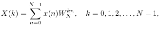
The DFT is defined by
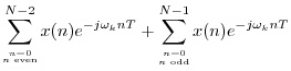
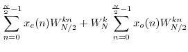
When ![]() is even, the DFT summation can be split into sums over the
odd and even indexes of the input signal:
is even, the DFT summation can be split into sums over the
odd and even indexes of the input signal:
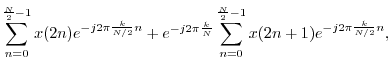
where
Radix 2 FFT
When ![]() is a power of
is a power of ![]() , say
, say ![]() where
where ![]() is an integer,
then the above DIT decomposition can be performed
is an integer,
then the above DIT decomposition can be performed ![]() times, until
each DFT is length
times, until
each DFT is length ![]() . A length
. A length ![]() DFT requires no multiplies. The
overall result is called a radix 2 FFT. A different radix 2
FFT is derived by performing decimation in frequency.
DFT requires no multiplies. The
overall result is called a radix 2 FFT. A different radix 2
FFT is derived by performing decimation in frequency.
A split radix FFT is theoretically more efficient than a pure radix 2 algorithm [73,31] because it minimizes real arithmetic operations. The term ``split radix'' refers to a DIT decomposition that combines portions of one radix 2 and two radix 4 FFTs [22].A.3On modern general-purpose processors, however, computation time is often not minimized by minimizing the arithmetic operation count (see §A.7 below).
Radix 2 FFT Complexity is N Log N
Putting together the length ![]() DFT from the
DFT from the ![]() length-
length-![]() DFTs in
a radix-2 FFT, the only multiplies needed are those used to combine
two small DFTs to make a DFT twice as long, as in Eq.
DFTs in
a radix-2 FFT, the only multiplies needed are those used to combine
two small DFTs to make a DFT twice as long, as in Eq.![]() (A.1).
Since there are approximately
(A.1).
Since there are approximately ![]() (complex) multiplies needed for each
stage of the DIT decomposition, and only
(complex) multiplies needed for each
stage of the DIT decomposition, and only ![]() stages of DIT (where
stages of DIT (where
![]() denotes the log-base-2 of
denotes the log-base-2 of ![]() ), we see that the total number
of multiplies for a length
), we see that the total number
of multiplies for a length ![]() DFT is reduced from
DFT is reduced from
![]() to
to
![]() , where
, where
![]() means ``on the order of
means ``on the order of ![]() ''. More
precisely, a complexity of
''. More
precisely, a complexity of
![]() means that given any
implementation of a length-
means that given any
implementation of a length-![]() radix-2 FFT, there exist a constant
radix-2 FFT, there exist a constant ![]() and integer
and integer ![]() such that the computational complexity
such that the computational complexity
![]() satisfies
satisfies
Fixed-Point FFTs and NFFTs
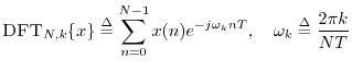
Recall (e.g., from Eq.![]() (6.1)) that the inverse DFT requires a
division by
(6.1)) that the inverse DFT requires a
division by ![]() that the forward DFT does not. In fixed-point
arithmetic (Appendix G), and when
that the forward DFT does not. In fixed-point
arithmetic (Appendix G), and when ![]() is a power of 2,
dividing by
is a power of 2,
dividing by ![]() may be carried out by right-shifting
may be carried out by right-shifting ![]() places in the binary word. Fixed-point implementations of the inverse
Fast Fourier Transforms (FFT) (Appendix A) typically right-shift one
place after each Butterfly stage. However, superior overall numerical
performance may be obtained by right-shifting after every other
butterfly stage [8], which corresponds to dividing both the
forward and inverse FFT by
places in the binary word. Fixed-point implementations of the inverse
Fast Fourier Transforms (FFT) (Appendix A) typically right-shift one
place after each Butterfly stage. However, superior overall numerical
performance may be obtained by right-shifting after every other
butterfly stage [8], which corresponds to dividing both the
forward and inverse FFT by ![]() (i.e.,
(i.e., ![]() is implemented
by half as many right shifts as dividing by
is implemented
by half as many right shifts as dividing by ![]() ). Thus, in
fixed-point, numerical performance can be improved, no extra work is
required, and the normalization work (right-shifting) is spread
equally between the forward and reverse transform, instead of
concentrating all
). Thus, in
fixed-point, numerical performance can be improved, no extra work is
required, and the normalization work (right-shifting) is spread
equally between the forward and reverse transform, instead of
concentrating all ![]() right-shifts in the inverse transform. The NDFT
is therefore quite attractive for fixed-point implementations.
right-shifts in the inverse transform. The NDFT
is therefore quite attractive for fixed-point implementations.
Because signal amplitude can grow by a factor of 2 from one butterfly
stage to the next, an extra guard bit is needed for each pair of
subsequent NDFT butterfly stages. Also note that if the DFT length
![]() is not a power of
is not a power of ![]() , the number of right-shifts in the
forward and reverse transform must differ by one (because
, the number of right-shifts in the
forward and reverse transform must differ by one (because
![]() is odd instead of even).
is odd instead of even).
Next Section:
Prime Factor Algorithm (PFA)
Previous Section:
Recommended Further Reading


