


Boundary Conditions as Perturbations
To study the effect of boundary conditions on the state transition
matrices
![]() and
and
![]() , it is convenient to write the terminated
transition matrix as the sum of of the ``left-clamped'' case
, it is convenient to write the terminated
transition matrix as the sum of of the ``left-clamped'' case
![]()
![]() (for which
(for which ![]() ) plus a series of one or more rank-one
perturbations. For example, introducing a right termination with
reflectance
) plus a series of one or more rank-one
perturbations. For example, introducing a right termination with
reflectance ![]() can be written
can be written
where
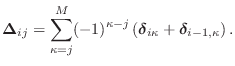
In general, when ![]() is odd, adding
is odd, adding
![]() to
to
![]()
![]() corresponds to a connection from left-going waves to
right-going waves, or vice versa (see Fig.E.2). When
corresponds to a connection from left-going waves to
right-going waves, or vice versa (see Fig.E.2). When ![]() is
odd and
is
odd and ![]() is even, the connection flows from the right-going to the
left-going signal path, thus providing a termination (or partial
termination) on the right. Left terminations flow from the bottom to
the top rail in Fig.E.2, and in such connections
is even, the connection flows from the right-going to the
left-going signal path, thus providing a termination (or partial
termination) on the right. Left terminations flow from the bottom to
the top rail in Fig.E.2, and in such connections ![]() is even
and
is even
and ![]() is odd. The spatial sample numbers involved in the connection
are
is odd. The spatial sample numbers involved in the connection
are
![]() and
and
![]() , where
, where
![]() denotes the greatest integer less than or equal to
denotes the greatest integer less than or equal to
![]() .
.
The rank-one perturbation of the DW transition matrix Eq.![]() (E.39)
corresponds to the following rank-one perturbation of the FDTD
transition matrix
(E.39)
corresponds to the following rank-one perturbation of the FDTD
transition matrix
![]()
![]() :
:
![\begin{displaymath}\mathbf{T}{\bm \delta}_{8,7}\mathbf{T}^{-1}
=
\left[\!
\begin...
...
0 & 0 & 0 & 0 & 0 & 0 & 1 & -1
\end{array}\!\right].
\protect\end{displaymath}](http://www.dsprelated.com/josimages_new/pasp/img4713.png)
In general, we have
Thus, the general rule is that
Next Section:
Reactive Terminations
Previous Section:
Resistive Terminations


