


Delay-Line Interpolation
As mentioned above, when an audio delay line needs to vary smoothly over time, some form of interpolation between samples is usually required to avoid ``zipper noise'' in the output signal as the delay length changes. There is a hefty literature on ``fractional delay'' in discrete-time systems, and the survey in [267] is highly recommended.
This section will describe the most commonly used cases. Linear interpolation is perhaps most commonly used because it is very straightforward and inexpensive, and because it sounds very good when the signal bandwidth is small compared with half the sampling rate. For a delay line in a nearly lossless feedback loop, such as in a vibrating string simulation, allpass interpolation is sometimes a better choice since it costs the same as linear interpolation in the first-order case and has no gain distortion. (Feedback loops can be very sensitive to gain distortions.) Finally, in later sections, some higher-order interpolation methods are described.
Linear Interpolation
Linear interpolation works by effectively drawing a straight line between two neighboring samples and returning the appropriate point along that line.
More specifically, let ![]() be a number between 0 and 1 which
represents how far we want to interpolate a signal
be a number between 0 and 1 which
represents how far we want to interpolate a signal ![]() between time
between time
![]() and time
and time ![]() . Then we can define the linearly interpolated
value
. Then we can define the linearly interpolated
value
![]() as follows:
as follows:
For
One-Multiply Linear Interpolation
Note that by factoring out ![]() , we can obtain a one-multiply
form,
, we can obtain a one-multiply
form,
Fractional Delay Filtering by Linear Interpolation
![\includegraphics[width=\twidth]{eps/delayli}](http://www.dsprelated.com/josimages_new/pasp/img934.png)
A linearly interpolated delay line is depicted in Fig.4.1. In
contrast to Eq.![]() (4.1), we interpolate linearly between times
(4.1), we interpolate linearly between times
![]() and
and ![]() , and
, and ![]() is called the fractional delay in
samples. The first-order (linear-interpolating) filter following the
delay line in Fig.4.1 may be called a fractional delay
filter [267]. Equation (4.1), on the other hand, expresses the more
general case of an interpolated table lookup, where
is called the fractional delay in
samples. The first-order (linear-interpolating) filter following the
delay line in Fig.4.1 may be called a fractional delay
filter [267]. Equation (4.1), on the other hand, expresses the more
general case of an interpolated table lookup, where ![]() is
regarded as a table of samples and
is
regarded as a table of samples and
![]() is regarded as an
interpolated table-lookup based on the samples stored at indices
is regarded as an
interpolated table-lookup based on the samples stored at indices ![]() and
and ![]() .
.
The difference between a fractional delay filter and an interpolated table lookup is that table-lookups can ``jump around,'' while fractional delay filters receive a sequential stream of input samples and produce a corresponding sequential stream of interpolated output values. As a result of this sequential access, fractional delay filters may be recursive IIR digital filters (provided the desired delay does not change too rapidly over time). In contrast, ``random-access'' interpolated table lookups are typically implemented using weighted linear combinations, making them equivalent to nonrecursive FIR filters in the sequential case.5.1
The C++ class implementing a linearly interpolated delay line in the Synthesis Tool Kit (STK) is called DelayL.
The frequency response of linear interpolation for fixed fractional
delay (![]() fixed in Fig.4.1) is shown in Fig.4.2.
From inspection of Fig.4.1, we see that linear interpolation is
a one-zero FIR filter. When used to provide a fixed fractional delay,
the filter is linear and time-invariant (LTI). When the fractional delay
fixed in Fig.4.1) is shown in Fig.4.2.
From inspection of Fig.4.1, we see that linear interpolation is
a one-zero FIR filter. When used to provide a fixed fractional delay,
the filter is linear and time-invariant (LTI). When the fractional delay ![]() changes over time, it is a linear time-varying filter.
changes over time, it is a linear time-varying filter.
![\includegraphics[width=\twidth]{eps/linear1}](http://www.dsprelated.com/josimages_new/pasp/img937.png) |
Linear interpolation sounds best when the signal is oversampled. Since natural audio spectra tend to be relatively concentrated at low frequencies, linear interpolation tends to sound very good at high sampling rates.
When interpolation occurs inside a feedback loop, such as in digital waveguide models for vibrating strings (see Chapter 6), errors in the amplitude response can be highly audible (particularly when the loop gain is close to 1, as it is for steel strings, for example). In these cases, it is possible to eliminate amplitude error (at some cost in delay error) by using an allpass filter for delay-line interpolation.
First-Order Allpass Interpolation
A delay line interpolated by a first-order allpass filter is drawn in Fig.4.3.
![\includegraphics[width=\twidth]{eps/delayai}](http://www.dsprelated.com/josimages_new/pasp/img938.png)
Intuitively, ramping the coefficients of the allpass gradually ``grows'' or ``hides'' one sample of delay. This tells us how to handle resets when crossing sample boundaries.
The difference equation is
![\begin{eqnarray*}
{\hat x}(n-\Delta) \isdef y(n) &=& \eta \cdot x(n) + x(n-1) - ...
...y(n-1) \\
&=& \eta \cdot \left[ x(n) - y(n-1)\right] + x(n-1).
\end{eqnarray*}](http://www.dsprelated.com/josimages_new/pasp/img939.png)
Thus, like linear interpolation, first-order allpass interpolation requires only one multiply and two adds per sample of output.
The transfer function is
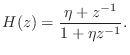
At low frequencies (
Figure 4.4 shows the phase delay of the first-order digital allpass filter for a variety of desired delays at dc. Since the amplitude response of any allpass is 1 at all frequencies, there is no need to plot it.
![\includegraphics[width=\twidth]{eps/allpass1}](http://www.dsprelated.com/josimages_new/pasp/img943.png)
The first-order allpass interpolator is generally controlled by
setting its dc delay to the desired delay. Thus, for a given desired
delay ![]() , the allpass coefficient is (from
Eq.
, the allpass coefficient is (from
Eq.![]() (4.3))
(4.3))

Note that, unlike linear interpolation, allpass interpolation is not suitable for ``random access'' interpolation in which interpolated values may be requested at any arbitrary time in isolation. This is because the allpass is recursive so that it must run for enough samples to reach steady state. However, when the impulse response is reasonably short, as it is for delays near one sample, it can in fact be used in ``random access mode'' by giving it enough samples with which to work.
![\includegraphics[width=4.8in]{eps/ap1pz}](http://www.dsprelated.com/josimages_new/pasp/img949.png)
The STK class implementing allpass-interpolated delay is DelayA.
Minimizing First-Order Allpass Transient Response
In addition to approaching a pole-zero cancellation at ![]() , another
undesirable artifact appears as
, another
undesirable artifact appears as
![]() : The transient
response also becomes long when the pole at
: The transient
response also becomes long when the pole at ![]() gets close to
the unit circle.
gets close to
the unit circle.
A plot of the impulse response for
![]() is shown in
Fig.4.6. We see a lot of ``ringing'' near half the sampling rate.
We actually should expect this from the nonlinear-phase
distortion which is clearly evident near half the sampling rate in
Fig.4.4. We can interpret this phenomenon as the signal
components near half the sampling rate being delayed by different
amounts than other frequencies, therefore ``sliding out of alignment''
with them.
is shown in
Fig.4.6. We see a lot of ``ringing'' near half the sampling rate.
We actually should expect this from the nonlinear-phase
distortion which is clearly evident near half the sampling rate in
Fig.4.4. We can interpret this phenomenon as the signal
components near half the sampling rate being delayed by different
amounts than other frequencies, therefore ``sliding out of alignment''
with them.
![\includegraphics[width=\twidth]{eps/ap1ir}](http://www.dsprelated.com/josimages_new/pasp/img952.png)
For audio applications, we would like to keep the impulse-response
duration short enough to sound ``instantaneous.'' That is, we do not
wish to have audible ``ringing'' in the time domain near ![]() . For
high quality sampling rates, such as larger than
. For
high quality sampling rates, such as larger than ![]() kHz, there
is no issue of direct audibility, since the ringing is above the range
of human hearing. However, it is often convenient, especially for
research prototyping, to work at lower sampling rates where
kHz, there
is no issue of direct audibility, since the ringing is above the range
of human hearing. However, it is often convenient, especially for
research prototyping, to work at lower sampling rates where ![]() is
audible. Also, many commercial products use such sampling rates to
save costs.
is
audible. Also, many commercial products use such sampling rates to
save costs.
Since the time constant of decay, in samples, of the impulse response
of a pole of radius ![]() is approximately
is approximately
For example, suppose 100 ms is chosen as the maximum ![]() allowed
at a sampling rate of
allowed
at a sampling rate of
![]() . Then applying the above constraints
yields
. Then applying the above constraints
yields
![]() , corresponding to the allowed delay range
, corresponding to the allowed delay range
![]() .
.
Linear Interpolation as Resampling
Convolution Interpretation
Linearly interpolated fractional delay is equivalent to filtering and resampling a weighted impulse train (the input signal samples) with a continuous-time filter having the simple triangular impulse response
![$\displaystyle h_l(t) = \left\{\begin{array}{ll} 1-\left\vert t/T\right\vert, & ...
...ght\vert\leq T, \\ [5pt] 0, & \hbox{otherwise}. \\ \end{array} \right. \protect$](http://www.dsprelated.com/josimages_new/pasp/img959.png)
Convolution of the weighted impulse train with
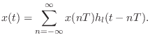
This continuous result can then be resampled at the desired fractional delay.
In discrete time processing, the operation Eq.![]() (4.5) can be
approximated arbitrarily closely by digital upsampling by a
large integer factor
(4.5) can be
approximated arbitrarily closely by digital upsampling by a
large integer factor ![]() , delaying by
, delaying by ![]() samples (an integer), then
finally downsampling by
samples (an integer), then
finally downsampling by ![]() , as depicted in Fig.4.7
[96]. The integers
, as depicted in Fig.4.7
[96]. The integers ![]() and
and ![]() are chosen so that
are chosen so that
![]() , where
, where ![]() the desired fractional delay.
the desired fractional delay.
![\includegraphics[width=0.8\twidth]{eps/polyphaseli}](http://www.dsprelated.com/josimages_new/pasp/img963.png)
The convolution interpretation of linear interpolation, Lagrange interpolation, and others, is discussed in [407].
Frequency Response of Linear Interpolation
Since linear interpolation can be expressed as a convolution of the
samples with a triangular pulse, we can derive the frequency
response of linear interpolation. Figure 4.7 indicates that
the triangular pulse ![]() serves as an anti-aliasing lowpass
filter for the subsequent downsampling by
serves as an anti-aliasing lowpass
filter for the subsequent downsampling by ![]() . Therefore, it should
ideally ``cut off'' all frequencies higher than
. Therefore, it should
ideally ``cut off'' all frequencies higher than ![]() .
.
Triangular Pulse as Convolution of Two Rectangular Pulses
The 2-sample wide triangular pulse ![]() (Eq.
(Eq.![]() (4.4)) can be
expressed as a convolution of the one-sample rectangular pulse with
itself.
(4.4)) can be
expressed as a convolution of the one-sample rectangular pulse with
itself.
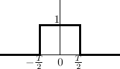
The one-sample rectangular pulse is shown in Fig.4.8 and may be defined analytically as
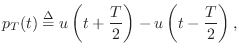
![$\displaystyle u(t) \isdef \left\{\begin{array}{ll}
1, & t\geq 0 \\ [5pt]
0, & t<0 \\
\end{array}\right..
$](http://www.dsprelated.com/josimages_new/pasp/img968.png)
Linear Interpolation Frequency Response
Since linear interpolation is a convolution of the samples with a
triangular pulse
![]() (from Eq.
(from Eq.![]() (4.5)),
the frequency response of the interpolation is given by the Fourier
transform
(4.5)),
the frequency response of the interpolation is given by the Fourier
transform ![]() , which yields a
sinc
, which yields a
sinc![]() function. This frequency
response applies to linear interpolation from discrete time to
continuous time. If the output of the interpolator is also sampled,
this can be modeled by sampling the continuous-time interpolation
result in Eq.
function. This frequency
response applies to linear interpolation from discrete time to
continuous time. If the output of the interpolator is also sampled,
this can be modeled by sampling the continuous-time interpolation
result in Eq.![]() (4.5), thereby aliasing the
sinc
(4.5), thereby aliasing the
sinc![]() frequency
response, as shown in Fig.4.9.
frequency
response, as shown in Fig.4.9.
![\includegraphics[width=3in]{eps/sincsquared}](http://www.dsprelated.com/josimages_new/pasp/img979.png)
In slightly more detail, from
![]() , and
, and
![]() sinc
sinc![]() , we have
, we have
The Fourier transform of ![]() is the same function aliased on
a block of size
is the same function aliased on
a block of size ![]() Hz. Both
Hz. Both ![]() and its alias are plotted
in Fig.4.9. The example in this figure pertains to an
output sampling rate which is
and its alias are plotted
in Fig.4.9. The example in this figure pertains to an
output sampling rate which is ![]() times that of the input signal.
In other words, the input signal is upsampled by a factor of
times that of the input signal.
In other words, the input signal is upsampled by a factor of ![]() using linear interpolation. The ``main lobe'' of the interpolation
frequency response
using linear interpolation. The ``main lobe'' of the interpolation
frequency response ![]() contains the original signal bandwidth;
note how it is attenuated near half the original sampling rate (
contains the original signal bandwidth;
note how it is attenuated near half the original sampling rate (![]() in Fig.4.9). The ``sidelobes'' of the frequency response
contain attenuated copies of the original signal bandwidth (see
the DFT stretch theorem), and thus constitute spectral imaging
distortion in the final output (sometimes also referred to as a kind
of ``aliasing,'' but, for clarity, that term will not be used for
imaging distortion in this book). We see that the frequency response
of linear interpolation is less than ideal in two ways:
in Fig.4.9). The ``sidelobes'' of the frequency response
contain attenuated copies of the original signal bandwidth (see
the DFT stretch theorem), and thus constitute spectral imaging
distortion in the final output (sometimes also referred to as a kind
of ``aliasing,'' but, for clarity, that term will not be used for
imaging distortion in this book). We see that the frequency response
of linear interpolation is less than ideal in two ways:
- The spectrum is ``rolled'' off near half the sampling rate. In fact, it is nowhere flat within the ``passband'' (-1 to 1 in Fig.4.9).
- Spectral imaging distortion is suppressed by only 26 dB (the level of the first sidelobe in Fig.4.9.
Special Cases
In the limiting case of ![]() , the input and output sampling rates are
equal, and all sidelobes of the frequency response
, the input and output sampling rates are
equal, and all sidelobes of the frequency response ![]() (partially
shown in Fig.4.9) alias into the main lobe.
(partially
shown in Fig.4.9) alias into the main lobe.
If the output is sampled at the same exact time instants as the input
signal, the input and output are identical. In terms of the aliasing
picture of the previous section, the frequency response aliases to a
perfect flat response over
![]() , with all spectral images
combining coherently under the flat gain. It is important in this
reconstruction that, while the frequency response of the underlying
continuous interpolating filter is aliased by sampling, the signal
spectrum is only imaged--not aliased; this is true for all positive
integers
, with all spectral images
combining coherently under the flat gain. It is important in this
reconstruction that, while the frequency response of the underlying
continuous interpolating filter is aliased by sampling, the signal
spectrum is only imaged--not aliased; this is true for all positive
integers ![]() and
and ![]() in Fig.4.7.
in Fig.4.7.
More typically, when linear interpolation is used to provide
fractional delay, identity is not obtained. Referring again to
Fig.4.7, with ![]() considered to be so large that it is
effectively infinite, fractional-delay by
considered to be so large that it is
effectively infinite, fractional-delay by ![]() can be modeled as
convolving the samples
can be modeled as
convolving the samples ![]() with
with
![]() followed by sampling
at
followed by sampling
at ![]() . In this case, a linear phase term has been introduced in
the interpolator frequency response, giving,
. In this case, a linear phase term has been introduced in
the interpolator frequency response, giving,
Large Delay Changes
When implementing large delay length changes (by many samples), a useful implementation is to cross-fade from the initial delay line configuration to the new configuration:
- Computational requirements are doubled during the cross-fade.
- The cross-fade should occur over a time interval long enough to yield a smooth result.
- The new delay interpolation filter, if any, may be initialized in advance
of the cross-fade, for maximum smoothness. Thus, if the transient
response of the interpolation filter is
 samples, the new delay-line
+ interpolation filter can be ``warmed up'' (executed) for
time steps before beginning the cross-fade. If the cross-fade time
is long compared with the interpolation filter duration, ``pre-warming''
is not necessary.
samples, the new delay-line
+ interpolation filter can be ``warmed up'' (executed) for
time steps before beginning the cross-fade. If the cross-fade time
is long compared with the interpolation filter duration, ``pre-warming''
is not necessary.
- This is not a true ``morph'' from one delay length to another since we do not pass through the intermediate delay lengths. However, it avoids a potentially undesirable Doppler effect.
- A single delay line can be shared such that the cross-fade occurs from one read-pointer (plus associated filtering) to another.
Next Section:
Lagrange Interpolation
Previous Section:
FDN Reverberation


