


FDNs as Digital Waveguide Networks
This section supplements §2.7 on Feedback Delay Networks in the context of digital waveguide theory. Specifically, we review the interpretation of an FDN as a special case of a digital waveguide network, summarizing [463,464,385].
Figure C.36 illustrates an ![]() -branch DWN. It consists of a single
scattering junction, indicated by a white circle, to which
-branch DWN. It consists of a single
scattering junction, indicated by a white circle, to which ![]() branches are connected. The far end of each branch is terminated by an
ideal non-inverting reflection (black circle). The waves traveling
into the junction are associated with the FDN delay line outputs
branches are connected. The far end of each branch is terminated by an
ideal non-inverting reflection (black circle). The waves traveling
into the junction are associated with the FDN delay line outputs
![]() , and the length of each waveguide is
half the length of the corresponding FDN delay line
, and the length of each waveguide is
half the length of the corresponding FDN delay line ![]() (since a traveling wave must traverse the branch twice to complete a
round trip from the junction to the termination and back). When
(since a traveling wave must traverse the branch twice to complete a
round trip from the junction to the termination and back). When ![]() is odd, we may replace the reflecting termination by a unit-sample
delay.
is odd, we may replace the reflecting termination by a unit-sample
delay.
![\includegraphics[scale=0.5]{eps/DWN}](http://www.dsprelated.com/josimages_new/pasp/img4051.png) |
Lossless Scattering
The delay-line inputs (outgoing traveling waves) are computed by
multiplying the delay-line outputs (incoming traveling waves) by the
![]() feedback matrix (scattering matrix)
feedback matrix (scattering matrix)
![]() . By
defining
. By
defining
![]() ,
,
![]() , we obtain the more
usual DWN notation
, we obtain the more
usual DWN notation
where
The junction of ![]() physical waveguides determines the structure of the
matrix
physical waveguides determines the structure of the
matrix
![]() according to the basic principles of physics.
according to the basic principles of physics.
Considering the parallel junction of ![]() lossless acoustic tubes, each
having characteristic admittance
lossless acoustic tubes, each
having characteristic admittance
![]() , the continuity of pressure and
conservation of volume velocity at the junction give us the following
scattering matrix for the pressure waves [433]:
, the continuity of pressure and
conservation of volume velocity at the junction give us the following
scattering matrix for the pressure waves [433]:
![$\displaystyle {\bf A} = \left[ \begin{array}{rrrr} \frac{2 \Gamma_{1}}{\Gamma_J...
...{2}}{\Gamma_J} & \dots & \frac{2 \Gamma_{N}}{\Gamma_J} -1\\ \end{array} \right]$](http://www.dsprelated.com/josimages_new/pasp/img4059.png)
where
 |
(C.121) |
Equation (C.121) can be derived by first writing the volume velocity at the

Normalized Scattering
For ideal numerical scaling in the ![]() sense, we may choose to propagate
normalized waves which lead to normalized scattering junctions
analogous to those encountered in normalized ladder filters [297].
Normalized waves may be either normalized pressure
sense, we may choose to propagate
normalized waves which lead to normalized scattering junctions
analogous to those encountered in normalized ladder filters [297].
Normalized waves may be either normalized pressure
![]() or normalized velocity
or normalized velocity
![]() . Since the signal power associated with a traveling
wave is simply
. Since the signal power associated with a traveling
wave is simply
![]() ,
they may also be called root-power waves [432].
Appendix C develops this topic in more detail.
,
they may also be called root-power waves [432].
Appendix C develops this topic in more detail.
The scattering matrix for normalized pressure waves is given by
![$\displaystyle \tilde{\mathbf{A}}= \left[ \begin{array}{llll} \frac{2 \Gamma_{1}...
..._{2}}}{\Gamma_J} & \dots & \frac{2 \Gamma_{n}}{\Gamma_J} -1 \end{array} \right]$](http://www.dsprelated.com/josimages_new/pasp/img4066.png)
The normalized scattering matrix can be expressed as a negative Householder reflection
where
General Conditions for Losslessness
The scattering matrices for lossless physical waveguide junctions give an apparently unexplored class of lossless FDN prototypes. However, this is just a subset of all possible lossless feedback matrices. We are therefore interested in the most general conditions for losslessness of an FDN feedback matrix. The results below are adapted from [463,385].
Consider the general case in which
![]() is allowed to be any
scattering matrix, i.e., it is associated with a
not-necessarily-physical junction of
is allowed to be any
scattering matrix, i.e., it is associated with a
not-necessarily-physical junction of ![]() physical waveguides.
Following the definition of losslessness in classical network theory,
we may say that a waveguide scattering matrix
physical waveguides.
Following the definition of losslessness in classical network theory,
we may say that a waveguide scattering matrix
![]() is said to be
lossless if the total complex power
[35] at the junction is scattering invariant, i.e.,
is said to be
lossless if the total complex power
[35] at the junction is scattering invariant, i.e.,
where
The following theorem gives a general characterization of lossless scattering:
Theorem: A scattering matrix (FDN feedback matrix)
![]() is
lossless if and only if its eigenvalues lie on the unit circle and its
eigenvectors are linearly independent.
is
lossless if and only if its eigenvalues lie on the unit circle and its
eigenvectors are linearly independent.
Proof: Since
![]() is positive definite, it can be factored (by
the Cholesky factorization) into the form
is positive definite, it can be factored (by
the Cholesky factorization) into the form
![]() , where
, where
![]() is an upper triangular matrix, and
is an upper triangular matrix, and
![]() denotes the Hermitian
transpose of
denotes the Hermitian
transpose of
![]() , i.e.,
, i.e.,
![]() . Since
. Since
![]() is
positive definite,
is
positive definite,
![]() is nonsingular and can be used as a
similarity transformation matrix. Applying the Cholesky decomposition
is nonsingular and can be used as a
similarity transformation matrix. Applying the Cholesky decomposition
![]() in Eq.
in Eq.![]() (C.125) yields
(C.125) yields
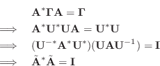
where
![]() , and
, and
Conversely, assume
![]() for each eigenvalue of
for each eigenvalue of
![]() , and
that there exists a matrix
, and
that there exists a matrix
![]() of linearly independent
eigenvectors of
of linearly independent
eigenvectors of
![]() . The matrix
. The matrix
![]() diagonalizes
diagonalizes
![]() to give
to give
![]() , where
, where
![]() diag
diag![]() . Taking the Hermitian transform of
this equation gives
. Taking the Hermitian transform of
this equation gives
![]() . Multiplying, we
obtain
. Multiplying, we
obtain
![]() . Thus, (C.125) is satisfied for
. Thus, (C.125) is satisfied for
![]() which is Hermitian and positive
definite.
which is Hermitian and positive
definite. ![]()
Thus, lossless scattering matrices may be fully parametrized as
![]() , where
, where
![]() is any unit-modulus diagonal
matrix, and
is any unit-modulus diagonal
matrix, and
![]() is any invertible matrix. In the real case, we
have
is any invertible matrix. In the real case, we
have
![]() diag
diag![]() and
and
![]() .
.
Note that not all lossless scattering matrices have a simple
physical interpretation as a scattering matrix for an
intersection of ![]() lossless reflectively terminated waveguides. In
addition to these cases (generated by all non-negative branch
impedances), there are additional cases corresponding to sign flips
and branch permutations at the junction. In terms of classical
network theory [35], such additional cases can be seen as
arising from the use of ``gyrators'' and/or ``circulators'' at the
scattering junction
[433]).
lossless reflectively terminated waveguides. In
addition to these cases (generated by all non-negative branch
impedances), there are additional cases corresponding to sign flips
and branch permutations at the junction. In terms of classical
network theory [35], such additional cases can be seen as
arising from the use of ``gyrators'' and/or ``circulators'' at the
scattering junction
[433]).
Next Section:
Waveguide Transformers and Gyrators
Previous Section:
Digital Waveguide Mesh


