


Frequency-Response Matching Using
Digital Filter Design Methods
Given force inputs and velocity outputs, the frequency response
of an ideal mass was given in Eq.![]() (7.1.2) as
(7.1.2) as
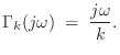
where we assume
Ideal Differentiator (Spring Admittance)
Figure 8.1 shows a graph of the frequency response of the
ideal differentiator (spring admittance). In principle, a
digital differentiator is a filter whose frequency response
![]() optimally approximates
optimally approximates ![]() for
for ![]() between
between ![]() and
and ![]() . Similarly, a digital integrator must
match
. Similarly, a digital integrator must
match ![]() along the unit circle in the
along the unit circle in the ![]() plane. The reason
an exact match is not possible is that the ideal frequency responses
plane. The reason
an exact match is not possible is that the ideal frequency responses
![]() and
and ![]() , when wrapped along the unit circle in the
, when wrapped along the unit circle in the
![]() plane, are not ``smooth'' functions any more (see
Fig.8.1). As a result, there is no filter with a
rational transfer function (i.e., finite order) that can match the
desired frequency response exactly.
plane, are not ``smooth'' functions any more (see
Fig.8.1). As a result, there is no filter with a
rational transfer function (i.e., finite order) that can match the
desired frequency response exactly.
![\includegraphics[scale=0.9]{eps/f_ideal_diff_fr_cropped}](http://www.dsprelated.com/josimages_new/pasp/img1805.png) |
The discontinuity at ![]() alone is enough to ensure that no
finite-order digital transfer function exists with the desired
frequency response. As with bandlimited interpolation (§4.4),
it is good practice to reserve a ``guard band'' between the highest
needed frequency
alone is enough to ensure that no
finite-order digital transfer function exists with the desired
frequency response. As with bandlimited interpolation (§4.4),
it is good practice to reserve a ``guard band'' between the highest
needed frequency
![]() (such as the limit of human hearing) and half
the sampling rate
(such as the limit of human hearing) and half
the sampling rate ![]() . In the guard band
. In the guard band
![]() , digital
filters are free to smoothly vary in whatever way gives the best
performance across frequencies in the audible band
, digital
filters are free to smoothly vary in whatever way gives the best
performance across frequencies in the audible band
![]() at the
lowest cost. Figure 8.2 shows an example.
Note that, as with filters used for bandlimited
interpolation, a small increment in oversampling factor yields a much
larger decrease in filter cost (when the sampling rate is near
at the
lowest cost. Figure 8.2 shows an example.
Note that, as with filters used for bandlimited
interpolation, a small increment in oversampling factor yields a much
larger decrease in filter cost (when the sampling rate is near
![]() ).
).
In the general case of Eq.![]() (8.14) with
(8.14) with ![]() , digital filters
can be designed to implement arbitrarily accurate admittance transfer
functions by finding an optimal rational approximation to the complex
function of a single real variable
, digital filters
can be designed to implement arbitrarily accurate admittance transfer
functions by finding an optimal rational approximation to the complex
function of a single real variable ![]()
Digital Filter Design Overview
This section (adapted from [428]), summarizes some of the more commonly used methods for digital filter design aimed at matching a nonparametric frequency response, such as typically obtained from input/output measurements. This problem should be distinguished from more classical problems with their own specialized methods, such as designing lowpass, highpass, and bandpass filters [343,362], or peak/shelf equalizers [559,449], and other utility filters designed from a priori mathematical specifications.
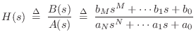
The problem of fitting a digital filter to a prescribed frequency
response may be formulated as follows. To simplify, we set ![]() .
.
Given a continuous complex function
![]() ,
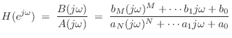
corresponding to a causal desired frequency response,9.8 find a stable digital filter of the form
,
corresponding to a causal desired frequency response,9.8 find a stable digital filter of the form
| (9.15) | |||
| (9.16) |
with
![]() given, such that some norm of the error
given, such that some norm of the error
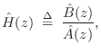
is minimum with respect to the filter coefficients
The approximate filter ![]() is typically constrained to be
stable, and since
is typically constrained to be
stable, and since
![]() is causal (no positive powers of
is causal (no positive powers of ![]() ),
stability implies causality. Consequently, the impulse response of the
model
),
stability implies causality. Consequently, the impulse response of the
model
![]() is zero for
is zero for ![]() .
.
The filter-design problem is then to find a (strictly) stable
![]() -pole,
-pole,
![]() -zero digital filter which minimizes some norm of
the error in the frequency-response. This is fundamentally
rational approximation of a complex function of a real
(frequency) variable, with constraints on the poles.
-zero digital filter which minimizes some norm of
the error in the frequency-response. This is fundamentally
rational approximation of a complex function of a real
(frequency) variable, with constraints on the poles.
While the filter-design problem has been formulated quite naturally,
it is difficult to solve in practice. The strict stability assumption
yields a compact space of filter coefficients
![]() , leading to the
conclusion that a best approximation
, leading to the
conclusion that a best approximation
![]() exists over this
domain.9.9Unfortunately, the norm of the error
exists over this
domain.9.9Unfortunately, the norm of the error
![]() typically is
not a convex9.10function of the filter coefficients on
typically is
not a convex9.10function of the filter coefficients on
![]() . This
means that algorithms based on gradient descent may fail to find an
optimum filter due to their premature termination at a suboptimal
local minimum of
. This
means that algorithms based on gradient descent may fail to find an
optimum filter due to their premature termination at a suboptimal
local minimum of
![]() .
.
Fortunately, there is at least one norm whose global minimization may be accomplished in a straightforward fashion without need for initial guesses or ad hoc modifications of the complex (phase-sensitive) IIR filter-design problem--the Hankel norm [155,428,177,36]. Hankel norm methods for digital filter design deliver a spontaneously stable filter of any desired order without imposing coefficient constraints in the algorithm.
An alternative to Hankel-norm approximation is to reformulate the
problem, replacing Eq.![]() (8.17) with a modified error criterion so that
the resulting problem can be solved by linear least-squares or
convex optimization techniques. Examples include
(8.17) with a modified error criterion so that
the resulting problem can be solved by linear least-squares or
convex optimization techniques. Examples include
- Pseudo-norm minimization:
(Pseudo-norms can be zero for nonzero functions.)
For example, Padé approximation falls in this category.
In Padé approximation, the first
 samples
of the impulse-response
samples
of the impulse-response  of
of  are matched exactly,
and the error in the remaining impulse-response samples is ignored.
are matched exactly,
and the error in the remaining impulse-response samples is ignored.
- Ratio Error: Minimize
 subject to
 . Minimizing the
  norm of the ratio error
yields the class of methods known as linear prediction
techniques [20,296,297]. Since,
by the definition of a norm, we have
norm of the ratio error
yields the class of methods known as linear prediction
techniques [20,296,297]. Since,
by the definition of a norm, we have
 ,
it follows that
,
it follows that
 ; therefore,
ratio error methods ignore the phase of the
approximation. It is also evident that ratio error is
minimized by making
; therefore,
ratio error methods ignore the phase of the
approximation. It is also evident that ratio error is
minimized by making
 larger than
 .9.11 For this reason, ratio-error
methods are considered most appropriate for modeling the
spectral envelope of
. It is well known
that these methods are fast and exceedingly robust in
practice, and this explains in part why they are used almost
exclusively in some data-intensive applications such as speech
modeling and other spectral-envelope applications. In some
applications, such as adaptive control or forecasting, the
fact that linear prediction error is minimized can justify
their choice.
.9.11 For this reason, ratio-error
methods are considered most appropriate for modeling the
spectral envelope of
. It is well known
that these methods are fast and exceedingly robust in
practice, and this explains in part why they are used almost
exclusively in some data-intensive applications such as speech
modeling and other spectral-envelope applications. In some
applications, such as adaptive control or forecasting, the
fact that linear prediction error is minimized can justify
their choice.
- Equation error: Minimize
When the
![$\displaystyle \left\Vert\,{\hat A}(e^{j\omega})H(e^{j\omega})-{\hat B}(e^{j\ome...
...}(e^{j\omega})\left[ H(e^{j\omega})-{\hat H}(e^{j\omega})\right]\,\right\Vert.
$](http://www.dsprelated.com/josimages_new/pasp/img1848.png) norm of equation-error is minimized, the
problem becomes solving a set of
norm of equation-error is minimized, the
problem becomes solving a set of
 linear
equations.
linear
equations.
The above expression makes it clear that equation-error can be seen as a frequency-response error weighted by
 . Thus, relatively large errors can be
expected where the poles of the optimum approximation (roots
of
. Thus, relatively large errors can be
expected where the poles of the optimum approximation (roots
of
 ) approach the unit circle
  . While this may
make the frequency-domain formulation seem ill-posed, in the
time-domain, linear prediction error is minimized in
the sense, and in certain applications this is ideal.
(Equation-error methods thus provide a natural extension of
ratio-error methods to include zeros.) Using so-called
Steiglitz-McBride iterations
[287,449,288], the
equation-error solution iteratively approaches the
norm-minimizing solution of Eq.
. While this may
make the frequency-domain formulation seem ill-posed, in the
time-domain, linear prediction error is minimized in
the sense, and in certain applications this is ideal.
(Equation-error methods thus provide a natural extension of
ratio-error methods to include zeros.) Using so-called
Steiglitz-McBride iterations
[287,449,288], the
equation-error solution iteratively approaches the
norm-minimizing solution of Eq. (8.17) for the L2
norm.
(8.17) for the L2
norm.
Examples of minimizing equation error using the matlab function invfreqz are given in §8.6.3 and §8.6.4 below. See [449, Appendix I] (based on [428, pp. 48-50]) for a discussion of equation-error IIR filter design and a derivation of a fast equation-error method based on the Fast Fourier Transform (FFT) (used in invfreqz).
- Conversion to real-valued approximation: For
example, power spectrum matching, i.e., minimization of
 , is possible
using the Chebyshev or
, is possible
using the Chebyshev or
 norm [428]. Similarly,
linear-phase filter design can be carried out with some
guarantees, since again the problem reduces to real-valued
approximation on the unit circle. The essence of these
methods is that the phase-response is eliminated from
the error measure, as in the norm of the ratio error, in order
to convert a complex approximation problem into a real one.
Real rational approximation of a continuous curve appears to
be solved in principle only under the
norm
[373,374].
norm [428]. Similarly,
linear-phase filter design can be carried out with some
guarantees, since again the problem reduces to real-valued
approximation on the unit circle. The essence of these
methods is that the phase-response is eliminated from
the error measure, as in the norm of the ratio error, in order
to convert a complex approximation problem into a real one.
Real rational approximation of a continuous curve appears to
be solved in principle only under the
norm
[373,374].
- Decoupling poles and zeros: An effective example of
this approach is Kopec's method [428] which consists of
using ratio error to find the poles, computing the error
spectrum
 , inverting it, and fitting poles again (to
 ). There is a wide variety of methods which first
fit poles and then zeros. None of these methods produce
optimum filters, however, in any normal sense.
). There is a wide variety of methods which first
fit poles and then zeros. None of these methods produce
optimum filters, however, in any normal sense.
In addition to these modifications, sometimes it is necessary to
reformulate the problem in order to achieve a different goal. For
example, in some audio applications, it is desirable to minimize the
log-magnitude frequency-response error. This is due to the way
we hear spectral distortions in many circumstances. A technique which
accomplishes this objective to the first order in the
![]() norm is
described in [428].
norm is
described in [428].
Sometimes the most important spectral structure is confined to an interval of the frequency domain. A question arises as to how this structure can be accurately modeled while obtaining a cruder fit elsewhere. The usual technique is a weighting function versus frequency. An alternative, however, is to frequency-warp the problem using a first-order conformal map. It turns out a first-order conformal map can be made to approximate very well frequency-resolution scales of human hearing such as the Bark scale or ERB scale [459]. Frequency-warping is especially valuable for providing an effective weighting function connection for filter-design methods, such as the Hankel-norm method, that are intrinsically do not offer choice of a weighted norm for the frequency-response error.
There are several methods which produce
![]() instead of
instead of
![]() directly. A fast spectral factorization technique is
useful in conjunction with methods of this category [428].
Roughly speaking, a size
directly. A fast spectral factorization technique is
useful in conjunction with methods of this category [428].
Roughly speaking, a size
![]() polynomial factorization is replaced
by an FFT and a size
polynomial factorization is replaced
by an FFT and a size
![]() system of linear equations.
system of linear equations.
Digital Differentiator Design
We saw the ideal digital differentiator frequency response in
Fig.8.1, where it was noted that the discontinuity in
the response at
![]() made an ideal design unrealizable
(infinite order). Fortunately, such a design is not even needed in
practice, since there is invariably a guard band between the highest
supported frequency
made an ideal design unrealizable
(infinite order). Fortunately, such a design is not even needed in
practice, since there is invariably a guard band between the highest
supported frequency
![]() and half the sampling rate
and half the sampling rate ![]() .
.
![\includegraphics[width=\twidth]{eps/iirdiff-mag-phs-N0-M10}](http://www.dsprelated.com/josimages_new/pasp/img1861.png) |
Figure 8.2 illustrates a more practical design specification for the digital differentiator as well as the performance of a tenth-order FIR fit using invfreqz (which minimizes equation error) in Octave.9.12 The weight function passed to invfreqz was 1 from 0 to 20 kHz, and zero from 20 kHz to half the sampling rate (24 kHz). Notice how, as a result, the amplitude response follows that of the ideal differentiator until 20 kHz, after which it rolls down to a gain of 0 at 24 kHz, as it must (see Fig.8.1). Higher order fits yield better results. Using poles can further improve the results, but the filter should be checked for stability since invfreqz designs filters in the frequency domain and does not enforce stability.9.13
Fitting Filters to Measured Amplitude Responses
The preceding filter-design example digitized an ideal differentiator, which is an example of converting an LTI lumped modeling element into a digital filter while maximally preserving its frequency response over the audio band. Another situation that commonly arises is the need for a digital filter that matches a measured frequency response over the audio band.
Measured Amplitude Response
Figure 8.3 shows a plot of simulated amplitude-response measurements at 10 frequencies equally spread out between 100 Hz and 3 kHz on a log frequency scale. The ``measurements'' are indicated by circles. Each circle plots, for example, the output amplitude divided by the input amplitude for a sinusoidal input signal at that frequency [449]. These ten data points are then extended to dc and half the sampling rate, interpolated, and resampled to a uniform frequency grid (solid line in Fig.8.3), as needed for FFT processing. The details of these computations are listed in Fig.8.4. We will fit a four-pole, one-zero, digital-filter frequency-response to these data.9.14
![\includegraphics[width=\twidth]{eps/tmps2-G}](http://www.dsprelated.com/josimages_new/pasp/img1862.png) |
NZ = 1; % number of ZEROS in the filter to be designed NP = 4; % number of POLES in the filter to be designed NG = 10; % number of gain measurements fmin = 100; % lowest measurement frequency (Hz) fmax = 3000; % highest measurement frequency (Hz) fs = 10000; % discrete-time sampling rate Nfft = 512; % FFT size to use df = (fmax/fmin)^(1/(NG-1)); % uniform log-freq spacing f = fmin * df .^ (0:NG-1); % measurement frequency axis % Gain measurements (synthetic example = triangular amp response): Gdb = 10*[1:NG/2,NG/2:-1:1]/(NG/2); % between 0 and 10 dB gain % Must decide on a dc value. % Either use what is known to be true or pick something "maximally % smooth". Here we do a simple linear extrapolation: dc_amp = Gdb(1) - f(1)*(Gdb(2)-Gdb(1))/(f(2)-f(1)); % Must also decide on a value at half the sampling rate. % Use either a realistic estimate or something "maximally smooth". % Here we do a simple linear extrapolation. While zeroing it % is appealing, we do not want any zeros on the unit circle here. Gdb_last_slope = (Gdb(NG) - Gdb(NG-1)) / (f(NG) - f(NG-1)); nyq_amp = Gdb(NG) + Gdb_last_slope * (fs/2 - f(NG)); Gdbe = [dc_amp, Gdb, nyq_amp]; fe = [0,f,fs/2]; NGe = NG+2; % Resample to a uniform frequency grid, as required by ifft. % We do this by fitting cubic splines evaluated on the fft grid: Gdbei = spline(fe,Gdbe); % say `help spline' fk = fs*[0:Nfft/2]/Nfft; % fft frequency grid (nonneg freqs) Gdbfk = ppval(Gdbei,fk); % Uniformly resampled amp-resp figure(1); semilogx(fk(2:end-1),Gdbfk(2:end-1),'-k'); grid('on'); axis([fmin/2 fmax*2 -3 11]); hold('on'); semilogx(f,Gdb,'ok'); xlabel('Frequency (Hz)'); ylabel('Magnitude (dB)'); title(['Measured and Extrapolated/Interpolated/Resampled ',... 'Amplitude Response']); |
Desired Impulse Response
It is good to check that the desired impulse response is not overly
aliased in the time domain. The impulse-response for this example is
plotted in Fig.8.5. We see that it appears quite short
compared with the inverse FFT used to compute it. The script in
Fig.8.6 gives the details of this computation, and also
prints out a measure of ``time-limitedness'' defined as the ![]() norm of the outermost 20% of the impulse response divided by its
total
norm of the outermost 20% of the impulse response divided by its
total ![]() norm--this measure was reported to be
norm--this measure was reported to be ![]() % for this
example.
% for this
example.
![\includegraphics[width=\twidth]{eps/tmps2-ir}](http://www.dsprelated.com/josimages_new/pasp/img1864.png) |
Note also that the desired impulse response is noncausal. In fact, it is zero phase [449]. This is of course expected because the desired frequency response was real (and nonnegative).
Ns = length(Gdbfk); if Ns~=Nfft/2+1, error("confusion"); end
Sdb = [Gdbfk,Gdbfk(Ns-1:-1:2)]; % install negative-frequencies

S = 10 .^ (Sdb/20); % convert to linear magnitude
s = ifft(S); % desired impulse response
s = real(s); % any imaginary part is quantization noise
tlerr = 100*norm(s(round(0.9*Ns:1.1*Ns)))/norm(s);
disp(sprintf(['Time-limitedness check: Outer 20%% of impulse ' ...
              'response is %0.2f %% of total rms'],tlerr));
% = 0.02 percent
if tlerr>1.0 % arbitrarily set 1% as the upper limit allowed
  error('Increase Nfft and/or smooth Sdb');
end

figure(2);
plot(s,'-k'); grid('on');   title('Impulse Response');
xlabel('Time (samples)');   ylabel('Amplitude');
|
Converting the Desired Amplitude Response to Minimum Phase
Phase-sensitive filter-design methods such as the equation-error method implemented in invfreqz are normally constrained to produce filters with causal impulse responses.9.15 In cases such as this (phase-sensitive filter design when we don't care about phase--or don't have it), it is best to compute the minimum phase corresponding to the desired amplitude response [449].
As detailed in Fig.8.8, the minimum phase is constructed by the cepstral method [449].9.16
The four-pole, one-zero filter fit using invfreqz is shown in Fig.8.7.
![\includegraphics[width=\twidth]{eps/tmps2-Hh}](http://www.dsprelated.com/josimages_new/pasp/img1865.png) |
c = ifft(Sdb); % compute real cepstrum from log magnitude spectrum % Check aliasing of cepstrum (in theory there is always some): caliaserr = 100*norm(c(round(Ns*0.9:Ns*1.1)))/norm(c); disp(sprintf(['Cepstral time-aliasing check: Outer 20%% of ' ... 'cepstrum holds %0.2f %% of total rms'],caliaserr)); % = 0.09 percent if caliaserr>1.0 % arbitrary limit error('Increase Nfft and/or smooth Sdb to shorten cepstrum'); end % Fold cepstrum to reflect non-min-phase zeros inside unit circle: % If complex: % cf=[c(1),c(2:Ns-1)+conj(c(Nfft:-1:Ns+1)),c(Ns),zeros(1,Nfft-Ns)]; cf = [c(1), c(2:Ns-1)+c(Nfft:-1:Ns+1), c(Ns), zeros(1,Nfft-Ns)]; Cf = fft(cf); % = dB_magnitude + j * minimum_phase Smp = 10 .^ (Cf/20); % minimum-phase spectrum Smpp = Smp(1:Ns); % nonnegative-frequency portion wt = 1 ./ (fk+1); % typical weight fn for audio wk = 2*pi*fk/fs; [B,A] = invfreqz(Smpp,wk,NZ,NP,wt); Hh = freqz(B,A,Ns); figure(3); plot(fk,db([Smpp(:),Hh(:)])); grid('on'); xlabel('Frequency (Hz)'); ylabel('Magnitude (dB)'); title('Magnitude Frequency Response'); % legend('Desired','Filter'); |
Further Reading on Digital Filter Design
This section provided only a ``surface scratch'' into the large topic of digital filter design based on an arbitrary frequency response. The main goal here was to provide a high-level orientation and to underscore the high value of such an approach for encapsulating linear, time-invariant subsystems in a computationally efficient yet accurate form. Applied examples will appear in later chapters. We close this section with some pointers for further reading in the area of digital filter design.
Some good books on digital filter design in general include [343,362,289]. Also take a look at the various references in the help/type info for Matlab/Octave functions pertaining to filter design. Methods for FIR filter design (used in conjunction with FFT convolution) are discussed in Book IV [456], and the equation-error method for IIR filter design was introduced in Book II [449]. See [281,282] for related techniques applied to guitar modeling. See [454] for examples of using matlab functions invfreqz and invfreqs to fit filters to measured frequency-response data (specifically the wah pedal design example). Other filter-design tools can be found in the same website area.
The overview of methods in §8.6.2 above is elaborated in [428], including further method details, application to violin modeling, and literature pointers regarding the methods addressed. Some of this material was included in [449, Appendix I].
In Octave or Matlab, say lookfor filter to obtain a list of filter-related functions. Matlab has a dedicated filter-design toolbox (say doc filterdesign in Matlab). In many matlab functions (both Octave and Matlab), there are literature citations in the source code. For example, type invfreqz in Octave provides a URL to a Web page (from [449]) describing the FFT method for equation-error filter design.
Next Section:
Commuted Synthesis
Previous Section:
Modal Expansion


