


A Lossy 1D Wave Equation
In any real vibrating string, there are energy losses due to yielding
terminations, drag by the surrounding air, and internal friction within the
string. While losses in solids generally vary in a complicated way with
frequency, they can usually be well approximated by a small number of
odd-order terms added to the wave equation. In the simplest case, force is
directly proportional to transverse string velocity, independent of
frequency. If this proportionality constant is ![]() , we obtain the
modified wave equation
, we obtain the
modified wave equation
Thus, the wave equation has been extended by a ``first-order'' term, i.e., a term proportional to the first derivative of
Setting
![]() in the wave equation to find the relationship
between temporal and spatial frequencies in the eigensolution, the wave
equation becomes
in the wave equation to find the relationship
between temporal and spatial frequencies in the eigensolution, the wave
equation becomes
 |
|||
 |
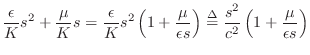
where
 |
(C.22) |
by the binomial theorem. For this small-loss approximation, we obtain the following relationship between temporal and spatial frequency:
| (C.23) |
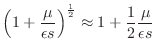
The eigensolution is then
| (C.24) |
The right-going part of the eigensolution is
| (C.25) |
which decays exponentially in the direction of propagation, and the left-going solution is
| (C.26) |
which also decays exponentially in the direction of travel.
Setting ![]() and using superposition to build up arbitrary traveling
wave shapes, we obtain the general class of solutions
and using superposition to build up arbitrary traveling
wave shapes, we obtain the general class of solutions
| (C.27) |
Sampling these exponentially decaying traveling waves at intervals of
![]() seconds (or
seconds (or ![]() meters) gives
meters) gives
The simulation diagram for the lossy digital waveguide is shown in Fig.C.5.
![\includegraphics[scale=0.9]{eps/floss}](http://www.dsprelated.com/josimages_new/pasp/img3340.png)
Again the discrete-time simulation of the decaying traveling-wave solution
is an exact implementation of the continuous-time solution at the
sampling positions and instants, even though losses are admitted in the
wave equation. Note also that the losses which are distributed in
the continuous solution have been consolidated, or lumped, at
discrete intervals of ![]() meters in the simulation. The loss factor
meters in the simulation. The loss factor
![]() summarizes the distributed loss incurred in one
sampling interval. The lumping of distributed losses does not introduce
an approximation error at the sampling points. Furthermore, bandlimited
interpolation can yield arbitrarily accurate reconstruction between
samples. The only restriction is again that all initial conditions and
excitations be bandlimited to below half the sampling rate.
summarizes the distributed loss incurred in one
sampling interval. The lumping of distributed losses does not introduce
an approximation error at the sampling points. Furthermore, bandlimited
interpolation can yield arbitrarily accurate reconstruction between
samples. The only restriction is again that all initial conditions and
excitations be bandlimited to below half the sampling rate.
Loss Consolidation
In many applications, it is possible to realize vast computational savings
in digital waveguide models by commuting losses out of unobserved and
undriven sections of the medium and consolidating them at a minimum number
of points. Because the digital simulation is linear and time invariant
(given constant medium parameters
![]() ), and because linear,
time-invariant elements commute, the diagram in Fig.C.6 is
exactly equivalent (to within numerical precision) to the previous diagram
in Fig.C.5.
), and because linear,
time-invariant elements commute, the diagram in Fig.C.6 is
exactly equivalent (to within numerical precision) to the previous diagram
in Fig.C.5.
![\includegraphics[scale=0.9]{eps/flloss}](http://www.dsprelated.com/josimages_new/pasp/img3343.png) |
Frequency-Dependent Losses
In nearly all natural wave phenomena, losses increase with frequency. Distributed losses due to air drag and internal bulk losses in the string tend to increase monotonically with frequency. Similarly, air absorption increases with frequency, adding loss for sound waves in acoustic tubes or open air [318].
Perhaps the apparently simplest modification to Eq.![]() (C.21) yielding
frequency-dependent damping is to add a third-order
time-derivative term [392]:
(C.21) yielding
frequency-dependent damping is to add a third-order
time-derivative term [392]:
While this model has been successful in practice [77], it turns out to go unstable at very high sampling rates. The technical term for this problem is that the PDE is ill posed [45].
A well posed replacement for Eq.![]() (C.28) is given by
(C.28) is given by
in which the third-order partial derivative with respect to time,
The solution of a lossy wave equation containing higher odd-order
derivatives with respect to time yields traveling waves which
propagate with frequency-dependent attenuation. Instead of scalar
factors ![]() distributed throughout the diagram as in Fig.C.5,
each
distributed throughout the diagram as in Fig.C.5,
each ![]() factor becomes a lowpass filter having some
frequency-response per sample denoted by
factor becomes a lowpass filter having some
frequency-response per sample denoted by ![]() . Because
propagation is passive, we will always have
. Because
propagation is passive, we will always have
![]() .
.
More specically, As shown in [392], odd-order partial derivatives with respect to time in the wave equation of the form

In view of the above, we see that we can add odd-order time
derivatives to the wave equation to approximate experimentally
observed frequency-dependent damping characteristics in vibrating
strings [73]. However, we then have the problem that
such wave equations are ill posed, leading to possible stability
failures at high sampling rates. As a result, it is generally
preferable to use mixed derivatives, as in Eq.![]() (C.29), and try to
achieve realistic damping using higher order spatial derivatives
instead.
(C.29), and try to
achieve realistic damping using higher order spatial derivatives
instead.
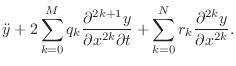
Well Posed PDEs for Modeling Damped Strings
A large class of well posed PDEs is given by [45]
Thus, to the ideal string wave equation Eq.
Digital Filter Models of Damped Strings
In an efficient digital simulation, lumped loss factors of the form
![]() are approximated by a rational frequency response
are approximated by a rational frequency response
![]() . In general, the coefficients of the optimal rational
loss filter are obtained by minimizing
. In general, the coefficients of the optimal rational
loss filter are obtained by minimizing
![]() with respect to the filter coefficients or the poles
and zeros of the filter. To avoid introducing frequency-dependent
delay, the loss filter should be a zero-phase,
finite-impulse-response (FIR) filter [362].
Restriction to zero phase requires the impulse response
with respect to the filter coefficients or the poles
and zeros of the filter. To avoid introducing frequency-dependent
delay, the loss filter should be a zero-phase,
finite-impulse-response (FIR) filter [362].
Restriction to zero phase requires the impulse response
![]() to
be finite in length (i.e., an FIR filter) and it must be symmetric
about time zero, i.e.,
to
be finite in length (i.e., an FIR filter) and it must be symmetric
about time zero, i.e.,
![]() . In most implementations,
the zero-phase FIR filter can be converted into a causal, linear
phase filter by reducing an adjacent delay line by half of the
impulse-response duration.
. In most implementations,
the zero-phase FIR filter can be converted into a causal, linear
phase filter by reducing an adjacent delay line by half of the
impulse-response duration.
Lossy Finite Difference Recursion
We will now derive a finite-difference model in terms of string displacement samples which correspond to the lossy digital waveguide model of Fig.C.5. This derivation generalizes the lossless case considered in §C.4.3.
Figure C.7 depicts a digital waveguide section once again in ``physical canonical form,'' as shown earlier in Fig.C.5, and introduces a doubly indexed notation for greater clarity in the derivation below [442,222,124,123].
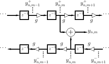
Referring to Fig.C.7, we have the following time-update relations:
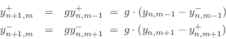
Adding these equations gives
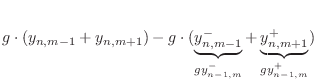
This is now in the form of the finite-difference time-domain (FDTD) scheme analyzed in [222]:
Frequency-Dependent Losses
The preceding derivation generalizes immediately to
frequency-dependent losses. First imagine each ![]() in Fig.C.7
to be replaced by
in Fig.C.7
to be replaced by ![]() , where for passivity we require
, where for passivity we require
![\begin{eqnarray*}
y^{+}_{n+1,m}&=& g\ast y^{+}_{n,m-1}\;=\; g\ast (y_{n,m-1}- y^...
...
&=& g\ast \left[(y_{n,m-1}+y_{n,m+1}) - g\ast y_{n-1,m}\right]
\end{eqnarray*}](http://www.dsprelated.com/josimages_new/pasp/img3373.png)
where ![]() denotes convolution (in the time dimension only).
Define filtered node variables by
denotes convolution (in the time dimension only).
Define filtered node variables by

Then the frequency-dependent FDTD scheme is simply
The frequency-dependent generalization of the FDTD scheme described in this section extends readily to the digital waveguide mesh. See §C.14.5 for the outline of the derivation.
Next Section:
The Dispersive 1D Wave Equation
Previous Section:
Sampled Traveling Waves


