


One-Port Network Theory
The basic idea of a one-port network [524] is shown in Fig. 7.5. The one-port is a ``black box'' with a single pair of input/output terminals, referred to as a port. A force is applied at the terminals and a velocity ``flows'' in the direction shown. The admittance ``seen'' at the port is called the driving point admittance. Network theory is normally described in terms of circuit theory elements, in which case a voltage is applied at the terminals and a current flows as shown. However, in our context, mechanical elements are preferable.
![\includegraphics[scale=0.9]{eps/loneport}](http://www.dsprelated.com/josimages_new/pasp/img1604.png) |
Series Combination of One-Ports
Figure 7.6 shows the series combination of two one-ports.
![\includegraphics[scale=0.9]{eps/lseries}](http://www.dsprelated.com/josimages_new/pasp/img1605.png)
Impedances add in series, so the aggregate impedance is
![]() , and the admittance is
, and the admittance is
Mass-Spring-Wall System
In a physical situation, if two elements are connected in such a way that they share a common velocity, then they are in series. An example is a mass connected to one end of a spring, where the other end is attached to a rigid support, and the force is applied to the mass, as shown in Fig. 7.7.
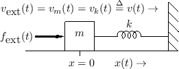
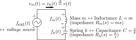
Figure 7.8 shows the electrical equivalent circuit corresponding to Fig.7.7.
 |
 |
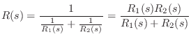
Parallel Combination of One-Ports
Figure Fig.7.10 shows the parallel combination of two one-ports.
![\includegraphics[scale=0.9]{eps/lparallel}](http://www.dsprelated.com/josimages_new/pasp/img1611.png) |
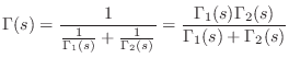
Admittances add in parallel, so the combined admittance is
![]() , and the impedance is
, and the impedance is
Spring-Mass System
When two physical elements are driven by a common force (yet
have independent velocities, as we'll soon see is quite possible),
they are formally in parallel. An example is a mass connected
to a spring in which the driving force is applied to one end of the
spring, and the mass is attached to the other end, as shown in
Fig.7.11. The compression force on the spring
is equal at all times to the rightward force on the mass. However,
the spring compression velocity ![]() does not always equal the
mass velocity
does not always equal the
mass velocity ![]() . We do have that the sum of the mass velocity
and spring compression velocity gives the velocity of the driving point,
i.e.,
. We do have that the sum of the mass velocity
and spring compression velocity gives the velocity of the driving point,
i.e.,
![]() . Thus, in a parallel connection, forces
are equal and velocities sum.
. Thus, in a parallel connection, forces
are equal and velocities sum.
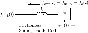
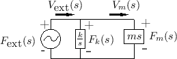
Figure 7.12 shows the electrical equivalent circuit corresponding to Fig.7.11.
 |
Mechanical Impedance Analysis
Impedance analysis is commonly used to analyze electrical circuits [110]. By means of equivalent circuits, we can use the same analysis methods for mechanical systems.
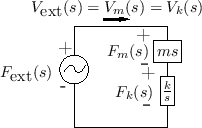
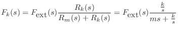
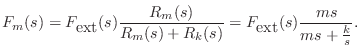
For example, referring to Fig.7.9, the Laplace transform of
the force on the spring ![]() is given by the so-called voltage
divider relation:8.2
is given by the so-called voltage
divider relation:8.2
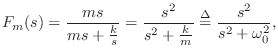
As a simple application, let's find the motion of the mass ![]() , after
time zero, given that the input force is an impulse at time 0:
, after
time zero, given that the input force is an impulse at time 0:
![\begin{eqnarray*}
V_m(s) &=& \frac{F_m(s)}{ms} \;=\; \frac{1}{m} \cdot \frac{s}{...
...}\right]\\ [5pt]
&\leftrightarrow& \frac{1}{m} \cos(\omega_0 t).
\end{eqnarray*}](http://www.dsprelated.com/josimages_new/pasp/img1626.png)
Thus, the impulse response of the mass oscillates sinusoidally with
radian frequency
![]() , and amplitude
, and amplitude ![]() . The
velocity starts out maximum at time
. The
velocity starts out maximum at time ![]() , which makes physical sense.
Also, the momentum transferred to the mass at time 0 is
, which makes physical sense.
Also, the momentum transferred to the mass at time 0 is
![]() ;
this is also expected physically because the time-integral of the applied
force is 1 (the area under any impulse
;
this is also expected physically because the time-integral of the applied
force is 1 (the area under any impulse ![]() is 1).
is 1).
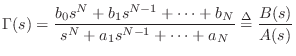
General One-Ports
An arbitrary interconnection of ![]() impedances and admittances, with input
and output force and/or velocities defined, results in a one-port with
admittance expressible as
impedances and admittances, with input
and output force and/or velocities defined, results in a one-port with
admittance expressible as
Passive One-Ports
It is well known that the impedance of every passive one-port is positive real (see §C.11.2). The reciprocal of a positive real function is positive real, so every passive impedance corresponds also to a passive admittance.
A complex-valued function of a complex variable ![]() is said to be
positive real (PR) if
is said to be
positive real (PR) if
- 1)
 is real whenever
  is real
- 2)
-
 whenever
 .
.
A particularly important property of positive real
functions is that the phase is bounded between plus and minus ![]() degrees, i.e.,
degrees, i.e.,
![\includegraphics[width=\twidth]{eps/interlace}](http://www.dsprelated.com/josimages_new/pasp/img1637.png) |
Referring to Fig.7.14, consider the graphical method for
computing phase response of a reactance from the pole zero diagram
[449].8.4Each zero on the positive ![]() axis contributes a net 90 degrees
of phase at frequencies above the zero. As frequency crosses the zero
going up, there is a switch from
axis contributes a net 90 degrees
of phase at frequencies above the zero. As frequency crosses the zero
going up, there is a switch from ![]() to
to ![]() degrees. For each
pole, the phase contribution switches from
degrees. For each
pole, the phase contribution switches from ![]() to
to ![]() degrees as
it is passed going up in frequency. In order to keep phase in
degrees as
it is passed going up in frequency. In order to keep phase in
![]() , it is clear that the poles and zeros must strictly
alternate. Moreover, all poles and zeros must be simple, since a
multiple poles or zero would swing the phase by more than
, it is clear that the poles and zeros must strictly
alternate. Moreover, all poles and zeros must be simple, since a
multiple poles or zero would swing the phase by more than ![]() degrees, and the reactance could not be positive real.
degrees, and the reactance could not be positive real.
The positive real property is fundamental to passive immittances and comes up often in the study of measured resonant systems. A practical modeling example (passive digital modeling of a guitar bridge) is discussed in §9.2.1.
Next Section:
Digitization of Lumped Models
Previous Section:
Impedance


