Piano Hammer Modeling

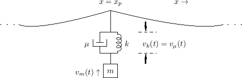
Free Books Physical Audio Signal Processing

The previous section treated an ideal point-mass striking an ideal string. This can be considered a simplified piano-hammer model. The model can be improved by adding a damped spring to the point-mass, as shown in Fig.9.22 (cf. Fig.9.12).

**Figure 9.22:** Ideal string excited by a mass and damped spring (a more realistic piano-hammer model).
$\includegraphics{eps/pianohammer}$

The impedance of this plucking system, as seen by the string, is the parallel combination of the mass impedance and the damped spring impedance $\mu+k/s$ . (The damper $\mu$ and spring are formally in series--see §7.2, for a refresher on series versus parallel connection.) Denoting the driving-point impedance of the hammer at the string contact-point by , we have

$\displaystyle R_h(s) \eqsp ms \left\Vert \left(\mu+\frac{k}{s}\right)\right. \eqsp \frac{\mu s^2 + ks}{s^2+\frac{\mu}{m}s+\frac{k}{m}}. \protect$

(10.19)

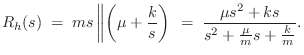
Thus, the scattering filters in the digital waveguide model are second order (biquads), while for the string struck by a mass (§9.3.1) we had first-order scattering filters. This is expected because we added another energy-storage element (a spring).

The impedance formulation of Eq. $\,$ (9.19) assumes all elements are linear and time-invariant (LTI), but in practice one can normally modulate element values as a function of time and/or state-variables and obtain realistic results for low-order elements. For this we must maintain filter-coefficient formulas that are explicit functions of physical state and/or time. For best results, state variables should be chosen so that any nonlinearities remain memoryless in the digitization [361,348,554,555].

Nonlinear Spring Model

In the musical acoustics literature, the piano hammer is classically modeled as a nonlinear spring [493,63,178,76,60,486,164].^10.14Specifically, the piano-hammer damping in Fig.9.22 is typically approximated by $\mu=0$ , and the spring is nonlinear and memoryless according to a simple power law:

$\displaystyle k(x_k) \; \approx \; Q_0\, x_k^{p-1}$

where

for a linear spring, and generally

for pianos. A fairly complete model across the piano keyboard (based on acoustic piano measurements) is as follows [487]:

$\begin{eqnarray*} Q_0 &=& 183\,e^{0.045\,n}\\ p &=& 3.7 + 0.015\,n\\ n &=& \mb... ...hammer-felt (nonlinear spring) compression}\\ v_k &=& \dot{x}_k \end{eqnarray*}$

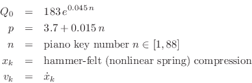
The upward force applied to the string by the hammer is therefore

$\displaystyle f_h(t) \eqsp Q_0\, x_k^p.$

(10.20)

This force is balanced at all times by the downward string force (string tension times slope difference), exactly as analyzed in §9.3.1 above.

Including Hysteresis

Since the compressed hammer-felt (wool) on real piano hammers shows significant hysteresis memory, an improved piano-hammer felt model is

$\displaystyle f_h(t) \eqsp Q_0\left[x_k^p + \alpha \frac{d(x_k^p)}{dt}\right], \protect$

(10.21)

where $\alpha = 248 + 1.83\,n - 5.5 \cdot 10^{-2}n^2$ ( $\mu$ s), and again

denotes piano key number [487].

Equation (9.21) is said to be a good approximation under normal playing conditions. A more complete hysteresis model is [487]

$\displaystyle f_h(t) \eqsp f_0\left[x_k^p(t) - \frac{\epsilon}{\tau_0} \int_0^t x_k^p(\xi) \exp\left(\frac{\xi-t}{\tau_0}\right)d\xi\right]$

where

$\begin{eqnarray*} f_0 &=& \mbox{ instantaneous hammer stiffness}\\ \epsilon &=&... ...resis parameter}\\ \tau_0 &=& \mbox{ hysteresis time constant}. \end{eqnarray*}$

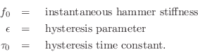
Relating to Eq. $\,$ (9.21) above, we have $Q_0=f_0\cdot(1-\epsilon)$ (N/mm $\null^p$ ).