


Pluck Modeling
The piano-hammer model of the previous section can also be configured
as a plectrum by making the mass and damping small or zero, and
by releasing the string when the contact force exceeds some threshold
![]() . That is, to a first approximation, a plectrum can be modeled
as a spring (linear or nonlinear) that disengages when either
it is far from the string or a maximum spring-force is exceeded. To
avoid discontinuities when the plectrum and string engage/disengage,
it is good to taper both the damping and spring-constant to zero at
the point of contact (as shown
below).
. That is, to a first approximation, a plectrum can be modeled
as a spring (linear or nonlinear) that disengages when either
it is far from the string or a maximum spring-force is exceeded. To
avoid discontinuities when the plectrum and string engage/disengage,
it is good to taper both the damping and spring-constant to zero at
the point of contact (as shown
below).
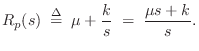
Starting with the piano-hammer impedance of Eq.![]() (9.19) and setting
the mass
(9.19) and setting
the mass ![]() to infinity (the plectrum holder is immovable), we define
the plectrum impedance as
to infinity (the plectrum holder is immovable), we define
the plectrum impedance as
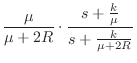
The force-wave reflectance of impedance ![]() in Eq.
in Eq.![]() (9.22), as
seen from the string, may be computed exactly as in
§9.3.1:
(9.22), as
seen from the string, may be computed exactly as in
§9.3.1:
![$\displaystyle \frac{\mbox{Impedance Step}}{\mbox{Impedance Sum}}
\eqsp \frac{[R_p(s)+R]-R}{[R_p(s)+R]+R}
\eqsp \frac{R_p(s)}{R_p(s)+2R}$](http://www.dsprelated.com/josimages_new/pasp/img2187.png)
If the spring damping is much greater than twice the string wave impedance (
Again following §9.3.1, the transmittance for force waves is given by
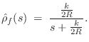
If the damping ![]() is set to zero, i.e., if the plectrum is to be modeled
as a simple linear spring, then the impedance becomes
is set to zero, i.e., if the plectrum is to be modeled
as a simple linear spring, then the impedance becomes
![]() ,
and the force-wave reflectance becomes
[128]
,
and the force-wave reflectance becomes
[128]
Digital Waveguide Plucked-String Model
When plucking a string, it is necessary to detect ``collisions''
between the plectrum and string. Also, more complete plucked-string
models will allow the string to ``buzz'' on the frets and ``slap''
against obstacles such as the fingerboard. For these reasons, it is
convenient to choose displacement waves for the waveguide
string model. The reflection and transmission filters for
displacement waves are the same as for velocity, namely,
![]() and
and
![]() .
.
As in the mass-string collision case, we obtain the one-filter
scattering-junction implementation shown in Fig.9.23. The filter
![]() may now be digitized using the bilinear transform as
previously (§9.3.1).
may now be digitized using the bilinear transform as
previously (§9.3.1).
Incorporating Control Motion
Let ![]() denote the vertical position of the mass
in Fig.9.22. (We still assume
denote the vertical position of the mass
in Fig.9.22. (We still assume ![]() .) We can think of
.) We can think of
![]() as the position of the control point on the
plectrum, e.g., the position of the ``pinch-point'' holding the
plectrum while plucking the string. In a harpsichord,
as the position of the control point on the
plectrum, e.g., the position of the ``pinch-point'' holding the
plectrum while plucking the string. In a harpsichord, ![]() can be
considered the jack position [347].
can be
considered the jack position [347].
Also denote by ![]() the rest length of the spring
the rest length of the spring ![]() in Fig.9.22, and let
in Fig.9.22, and let
![]() denote the
position of the ``end'' of the spring while not in contact with the
string. Then the plectrum makes contact with the string when
denote the
position of the ``end'' of the spring while not in contact with the
string. Then the plectrum makes contact with the string when
Let the subscripts ![]() and
and ![]() each denote one side of the scattering
system, as indicated in Fig.9.23. Then, for example,
each denote one side of the scattering
system, as indicated in Fig.9.23. Then, for example,
![]() is the displacement of the string on the left (side
is the displacement of the string on the left (side
![]() ) of plucking point, and
) of plucking point, and ![]() is on the right side of
is on the right side of ![]() (but
still located at point
(but
still located at point ![]() ). By continuity of the string, we have
). By continuity of the string, we have
When the spring engages the string (![]() ) and begins to compress,
the upward force on the string at the contact point is given by
) and begins to compress,
the upward force on the string at the contact point is given by
During contact, force equilibrium at the plucking point requires (cf. §9.3.1)
where
Substituting
![]() and taking the Laplace transform yields
and taking the Laplace transform yields
![$\displaystyle Y(s)
\eqsp Y_1^+(s) + Y_2^-(s) + \frac{1}{2R} \frac{F_k(s)}{s}
\eqsp Y_1^+(s) + Y_2^-(s) + \frac{k}{2Rs}\left[Y_e(s) - Y(s)\right].
$](http://www.dsprelated.com/josimages_new/pasp/img2224.png)
![\begin{eqnarray*}
Y(s) &=& \left[1-\hat{\rho}_f(s)\right]\cdot
\left[Y_1^+(s)+Y...
...)\cdot \left\{Y_e(s)
- \left[Y_1^+(s)+Y_2^-(s)\right]\right\},
\end{eqnarray*}](http://www.dsprelated.com/josimages_new/pasp/img2226.png)
where, as first noted at Eq.![]() (9.24) above,
(9.24) above,

![\begin{eqnarray*}
Y_d^+ &=& Y_e - \left(Y_1^+ + Y_2^-\right)\\ [5pt]
Y_1^- &=& Y...
...\hat{\rho}_f Y_d^+\\ [5pt]
Y_2^+ &=& Y_1^+ + \hat{\rho}_f Y_d^+.
\end{eqnarray*}](http://www.dsprelated.com/josimages_new/pasp/img2228.png)
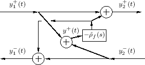
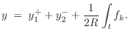
This system is diagrammed in Fig.9.24. The manipulation of the
minus signs relative to Fig.9.23 makes it convenient for
restricting ![]() to positive values only (as shown in the
figure), corresponding to the plectrum engaging the string going up.
This uses the approximation
to positive values only (as shown in the
figure), corresponding to the plectrum engaging the string going up.
This uses the approximation
![]() ,
which is exact when
,
which is exact when
![]() , i.e., when the plectrum does not affect
the string displacement at the current time. It is therefore exact at
the time of collision and also applicable just after release.
Similarly,
, i.e., when the plectrum does not affect
the string displacement at the current time. It is therefore exact at
the time of collision and also applicable just after release.
Similarly,
![]() can be used to trigger a release of the
string from the plectrum.
can be used to trigger a release of the
string from the plectrum.
Successive Pluck Collision Detection
As discussed above, in a simple 1D plucking model, the plectrum comes
up and engages the string when
![]() , and above some
maximum force the plectrum releases the string. At this point, it is
``above'' the string. To pluck again in the same direction, the
collision-detection must be disabled until we again have
, and above some
maximum force the plectrum releases the string. At this point, it is
``above'' the string. To pluck again in the same direction, the
collision-detection must be disabled until we again have ![]() ,
requiring one bit of state to keep track of that.10.16 The harpsichord jack
plucks the string only in the ``up'' direction due to its asymmetric
behavior in the two directions [143]. If only
``up picks'' are supported, then engagement can be suppressed after a
release until
,
requiring one bit of state to keep track of that.10.16 The harpsichord jack
plucks the string only in the ``up'' direction due to its asymmetric
behavior in the two directions [143]. If only
``up picks'' are supported, then engagement can be suppressed after a
release until ![]() comes back down below the envelope of string
vibration (e.g.,
comes back down below the envelope of string
vibration (e.g.,
![]() ). Note that
intermittent disengagements as a plucking cycle begins are normal;
there is often an audible ``buzzing'' or ``chattering'' when plucking
an already vibrating string.
). Note that
intermittent disengagements as a plucking cycle begins are normal;
there is often an audible ``buzzing'' or ``chattering'' when plucking
an already vibrating string.
When plucking up and down in alternation, as in the tremolo
technique (common on mandolins), the collision detection alternates
between ![]() and
and ![]() , and again a bit of state is needed to
keep track of which comparison to use.
, and again a bit of state is needed to
keep track of which comparison to use.
Plectrum Damping
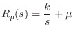
To include damping ![]() in the plectrum model, the load impedance
in the plectrum model, the load impedance
![]() goes back to Eq.
goes back to Eq.![]() (9.22):
(9.22):
Digitization of the Damped-Spring Plectrum
Applying the bilinear transformation (§7.3.2) to the reflectance
![]() in Eq.
in Eq.![]() (9.23) (including damping) yields the
following first-order digital force-reflectance filter:
(9.23) (including damping) yields the
following first-order digital force-reflectance filter:
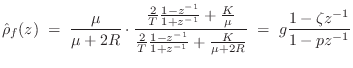
 (digital
  (digital zero)
The transmittance filter is again
Feathering
Since the pluck model is linear, the parameters are not signal-dependent. As a result, when the string and spring separate, there is a discontinuous change in the reflection and transmission coefficients. In practice, it is useful to ``feather'' the switch-over from one model to the next [470]. In this instance, one appealing choice is to introduce a nonlinear spring, as is commonly used for piano-hammer models (see §9.3.2 for details).
Let the nonlinear spring model take the form
The foregoing suggests a nonlinear tapering of the damping ![]() in
addition to the tapering the stiffness
in
addition to the tapering the stiffness ![]() as the spring compression
approaches zero. One natural choice would be
as the spring compression
approaches zero. One natural choice would be
In summary, the engagement and disengagement of the plucking system can be ``feathered'' by a nonlinear spring and damper in the plectrum model.
Next Section:
Stiff Piano Strings
Previous Section:
Piano Hammer Modeling


