


Rigid Terminations
A rigid termination is the simplest case of a string (or tube)
termination. It imposes the constraint that the string (or air) cannot move
at the termination. (We'll look at the more practical case of a yielding
termination in §9.2.1.) If we terminate a length ![]() ideal string at
ideal string at
![]() and
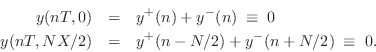
and ![]() , we then have the ``boundary conditions''
, we then have the ``boundary conditions''
where ``
Applying the traveling-wave decomposition from Eq.![]() (6.2), we have
(6.2), we have
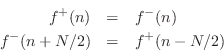
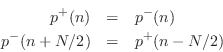
Therefore, solving for the reflected waves gives
| (7.10) | |||
| (7.11) |
A digital simulation diagram for the rigidly terminated ideal string is shown in Fig.6.3. A ``virtual pickup'' is shown at the arbitrary location
![\includegraphics[width=\twidth]{eps/fterminatedstring}](http://www.dsprelated.com/josimages_new/pasp/img1360.png) |
Velocity Waves at a Rigid Termination
Since the displacement is always zero at a rigid termination, the velocity is also zero there:
Such inverting reflections for velocity waves at a rigid termination are identical for models of vibrating strings and acoustic tubes.
Force or Pressure Waves at a Rigid Termination
To find out how force or pressure waves recoil from a rigid
termination, we may convert velocity waves to force or velocity waves
by means of the Ohm's law relations of Eq.![]() (6.6) for strings
(or Eq.
(6.6) for strings
(or Eq.![]() (6.7) for acoustic tubes), and then use
Eq.
(6.7) for acoustic tubes), and then use
Eq.![]() (6.12), and then Eq.
(6.12), and then Eq.![]() (6.6) again:
(6.6) again:

Thus, force (and pressure) waves reflect from a rigid termination with no sign inversion:7.3
The reflections from a rigid termination in a digital-waveguide acoustic-tube simulation are exactly analogous:
Waveguide terminations in acoustic stringed and wind instruments are never perfectly rigid. However, they are typically passive, which means that waves at each frequency see a reflection coefficient not exceeding 1 in magnitude. Aspects of passive ``yielding'' terminations are discussed in §C.11.
Next Section:
Moving Rigid Termination
Previous Section:
Ideal Acoustic Tube


