


Traveling-Wave Solution
It is easily shown that the lossless 1D wave equation
![]() is solved by any string shape which travels to the left or right with
speed
is solved by any string shape which travels to the left or right with
speed
![]() . Denote right-going
traveling waves in general by
. Denote right-going
traveling waves in general by
![]() and left-going
traveling waves by
and left-going
traveling waves by
![]() , where
, where ![]() and
and ![]() are assumed
twice-differentiable.C.1Then a general class of solutions to the
lossless, one-dimensional, second-order wave equation can be expressed
as
are assumed
twice-differentiable.C.1Then a general class of solutions to the
lossless, one-dimensional, second-order wave equation can be expressed
as
The next section derives the result that
An important point to note about the traveling-wave solution of the 1D
wave equation is that a function of two variables ![]() has been
replaced by two functions of a single variable in time units. This
leads to great reductions in computational complexity.
has been
replaced by two functions of a single variable in time units. This
leads to great reductions in computational complexity.
The traveling-wave solution of the wave equation was first published by d'Alembert in 1747 [100]. See Appendix A for more on the history of the wave equation and related topics.
Traveling-Wave Partial Derivatives
Because we have defined our traveling-wave components
![]() and
and
![]() as having arguments in units of time, the partial
derivatives with respect to time
as having arguments in units of time, the partial
derivatives with respect to time ![]() are identical to simple
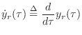
derivatives of these functions. Let
are identical to simple
derivatives of these functions. Let
![]() and
and
![]() denote the
(partial) derivatives with respect to time of
denote the
(partial) derivatives with respect to time of ![]() and
and ![]() ,
respectively. In contrast, the partial derivatives with respect to
,
respectively. In contrast, the partial derivatives with respect to ![]() are
are
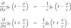
Denoting the spatial
partial derivatives by ![]() and
and
![]() , respectively, we can write more succinctly
, respectively, we can write more succinctly
![\begin{eqnarray*}
y'_r&=& -\frac{1}{c}{\dot y}_r\\ [5pt]
y'_l&=& \frac{1}{c}{\dot y}_l,
\end{eqnarray*}](http://www.dsprelated.com/josimages_new/pasp/img3234.png)
where this argument-free notation assumes the same ![]() and
and ![]() for all
terms in each equation, and the subscript
for all
terms in each equation, and the subscript ![]() or
or ![]() determines
whether the omitted argument is
determines
whether the omitted argument is ![]() or
or ![]() .
.
Now we can see that the second partial derivatives in ![]() are
are

These relations, together with the fact that partial differention is a linear operator, establish that
Use of the Chain Rule
These traveling-wave partial-derivative relations may be derived a bit
more formally by means of the chain rule from calculus, which
states that, for the composition of functions ![]() and
and ![]() , i.e.,
, i.e.,
To apply the chain rule to the spatial differentiation of traveling waves, define
![\begin{eqnarray*}
g_r(t,x) &=& t - \frac{x}{c}\\ [10pt]
g_l(t,x) &=& t + \frac{x}{c}.
\end{eqnarray*}](http://www.dsprelated.com/josimages_new/pasp/img3242.png)
Then the traveling-wave components can be written as
![]() and
and
![]() , and their partial derivatives with respect to
, and their partial derivatives with respect to ![]() become
become
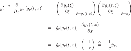
and similarly for ![]() .
.
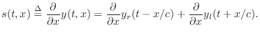
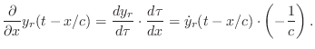
String Slope from Velocity Waves
Let's use the above result to derive the slope of the ideal
vibrating string
From Eq.![]() (C.11), we have the string displacement given by
(C.11), we have the string displacement given by
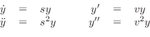
Wave Velocity
Because ![]() is an eigenfunction under differentiation
(i.e., the exponential function is its own derivative), it is often
profitable to replace it with a generalized exponential function, with
maximum degrees of freedom in its parametrization, to see if
parameters can be found to fulfill the constraints imposed by differential
equations.
is an eigenfunction under differentiation
(i.e., the exponential function is its own derivative), it is often
profitable to replace it with a generalized exponential function, with
maximum degrees of freedom in its parametrization, to see if
parameters can be found to fulfill the constraints imposed by differential
equations.
In the case of the one-dimensional ideal wave equation (Eq.![]() (C.1)),
with no boundary conditions, an appropriate choice of eigensolution is
(C.1)),
with no boundary conditions, an appropriate choice of eigensolution is
| (C.12) |
Substituting into the wave equation yields
| (C.13) | |||
 |
 |
||
Thus
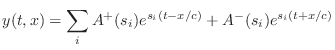
D'Alembert Derived
Setting
![]() , and extending the summation to an integral,
we have, by Fourier's theorem,
, and extending the summation to an integral,
we have, by Fourier's theorem,
for arbitrary continuous functions
An example of the appearance of the traveling wave components shortly after plucking an infinitely long string at three points is shown in Fig.C.2.
![\includegraphics[width=\twidth]{eps/f_t_waves_no_term}](http://www.dsprelated.com/josimages_new/pasp/img3269.png) |
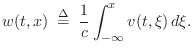
Converting Any String State to Traveling Slope-Wave Components
We verified in §C.3.1 above that traveling-wave components ![]() and
and ![]() in Eq.
in Eq.![]() (C.14) satisfy the ideal string wave equation
(C.14) satisfy the ideal string wave equation
![]() . By definition, the physical string displacement is
given by the sum of the traveling-wave components, or
. By definition, the physical string displacement is
given by the sum of the traveling-wave components, or
Thus, given any pair of traveling waves
The state of an ideal string at
time ![]() is classically specified by its displacement
is classically specified by its displacement ![]() and
velocity
and
velocity

![$\displaystyle \left[\begin{array}{c} y(t,x) \\ [2pt] v(t,x) \end{array}\right] ...
...ght]
\left[\begin{array}{c} y_r(t-x/c) \\ [2pt] y_l(t+x/c) \end{array}\right].
$](http://www.dsprelated.com/josimages_new/pasp/img3273.png)
![$\displaystyle \left[\begin{array}{c} y'^{+} \\ [2pt] y'^{-} \end{array}\right] ...
...eft[\begin{array}{c} y'-\frac{v}{c} \\ [2pt] y'+\frac{v}{c} \end{array}\right]
$](http://www.dsprelated.com/josimages_new/pasp/img3274.png)
![$\displaystyle \left[\begin{array}{c} y^{+} \\ [2pt] y^{-} \end{array}\right] \eqsp \frac{1}{2}\left[\begin{array}{c} y-w \\ [2pt] y+w \end{array}\right]
$](http://www.dsprelated.com/josimages_new/pasp/img3275.png)
It will be seen in §C.7.4 that state conversion between physical variables and traveling-wave components is simpler when force and velocity are chosen as the physical state variables (as opposed to displacement and velocity used here).
Next Section:
Sampled Traveling Waves
Previous Section:
The Finite Difference Approximation


