


The DFT Filter Bank
To obtain insight into the operation of filter banks implemented using an FFT, this section will derive the details of the DFT Filter Bank. More general STFT filter banks are obtained by using different windows and hop sizes, but otherwise are no different from the basic DFT filter bank.
The Discrete Fourier Transform (DFT) is defined by [264]
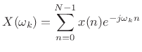 |
(10.4) |
where
 . In this section, we will show how the DFT can be computed
exactly from a bank of
. In this section, we will show how the DFT can be computed
exactly from a bank of
The Running-Sum Lowpass Filter
Perhaps the simplest FIR lowpass filter is the so-called
running-sum lowpass filter [175]. The impulse
response of the length ![]() running-sum lowpass filter is given by
running-sum lowpass filter is given by
![$\displaystyle h(n) \isdef \left\{\begin{array}{ll} 1, & n=0,1,2,...,N-1 \\ [5pt] 0, & \hbox{otherwise.} \\ \end{array} \right. \protect$](http://www.dsprelated.com/josimages_new/sasp2/img1568.png)
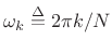
Figure 9.10 depicts the generic operation of filtering ![]() by
by ![]() to produce
to produce ![]() , where
, where ![]() is the impulse response of the
filter. The output signal is given by the convolution of
is the impulse response of the
filter. The output signal is given by the convolution of ![]() and
and ![]() :
:
In this form, it is clear why the filter (9.5) is called
``running sum'' filter. Dividing it by ![]() , it becomes a ``moving
average'' filter, averaging the most recent
, it becomes a ``moving
average'' filter, averaging the most recent ![]() input samples.
input samples.
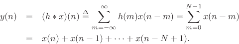
The transfer function of the running-sum filter is given by [263]
 |
(10.6) |
so that its frequency response is
![\begin{eqnarray*}
H(e^{j\omega}) &=& \frac{1-e^{-j\omega N}}{1-e^{-j\omega }}
= \frac{e^{-j\omega N/2}}{e^{-j\omega /2}}
\frac{\sin(\omega N/2)}{\sin(\omega /2)}\\ [10pt]
&\isdef &
Ne^{-j\omega(N-1)/2} \hbox{asinc}_N(\omega ).
\end{eqnarray*}](http://www.dsprelated.com/josimages_new/sasp2/img1572.png)
Recall that the term
![]() is a linear phase
term corresponding to a delay of
is a linear phase
term corresponding to a delay of ![]() samples (half of the FIR
filter order). This arises because we defined the running-sum lowpass
filter as a causal, linear phase filter.
samples (half of the FIR
filter order). This arises because we defined the running-sum lowpass
filter as a causal, linear phase filter.
We encountered the ``aliased sinc function''
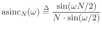 |
(10.7) |
previously in Chapter 5 (§3.1.2) and elsewhere as the Fourier transform (DTFT) of a sampled rectangular pulse (or rectangular window).
Note that the dc gain of the length ![]() running sum filter is
running sum filter is ![]() . We
could use a moving average instead of a running sum (
. We
could use a moving average instead of a running sum (
![]() ) to obtain unity dc gain.
) to obtain unity dc gain.
![\includegraphics[width=4in]{eps/sincabs}](http://www.dsprelated.com/josimages_new/sasp2/img1577.png)
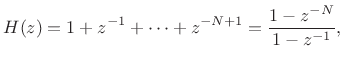
Figure 9.11 shows the amplitude response of the running-sum
lowpass filter for length ![]() . The gain at dc is
. The gain at dc is ![]() , and nulls
occur at
, and nulls
occur at
![]() and
and ![]() . These nulls occur
at the sinusoidal frequencies having respectively one and two periods
under the 5-sample ``rectangular window''. (Three periods would need
at least
. These nulls occur
at the sinusoidal frequencies having respectively one and two periods
under the 5-sample ``rectangular window''. (Three periods would need
at least
![]() samples, so
samples, so ![]() doesn't ``fit''.) Since
the pass-band about dc is not flat, it is better to call this a
``dc-pass filter'' rather than a ``lowpass filter.'' We could also
call it a dc sampling filter.10.1
doesn't ``fit''.) Since
the pass-band about dc is not flat, it is better to call this a
``dc-pass filter'' rather than a ``lowpass filter.'' We could also
call it a dc sampling filter.10.1
Modulation by a Complex Sinusoid
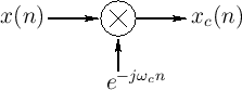
Figure 9.12 shows the system diagram for complex
demodulation.10.2The input signal ![]() is multiplied by a
complex sinusoid to produce the frequency-shifted result
is multiplied by a
complex sinusoid to produce the frequency-shifted result
| (10.8) |
Given a signal expressed as a sum of sinusoids,
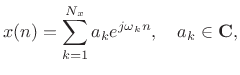 |
(10.9) |
then the demodulation produces
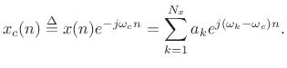 |
(10.10) |
We see that frequency
Making a Bandpass Filter from a Lowpass Filter
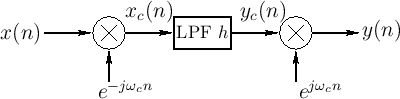 |
Figure 9.13 shows how a bandpass filter can be made using a lowpass
filter together with modulation. The input spectrum is
frequency-shifted by ![]() , lowpass filtered, then
frequency-shifted by
, lowpass filtered, then
frequency-shifted by ![]() , thereby creating a bandpass filter
centered at frequency
, thereby creating a bandpass filter
centered at frequency ![]() . From our experience with
rectangular-window transforms (Fig.9.11 being one example), we
can say that the bandpass-filter bandwidth is equal to the main-lobe
width of the aliased sinc function, or
. From our experience with
rectangular-window transforms (Fig.9.11 being one example), we
can say that the bandpass-filter bandwidth is equal to the main-lobe
width of the aliased sinc function, or ![]() radians per sample
(measured from zero-crossing to zero-crossing).
radians per sample
(measured from zero-crossing to zero-crossing).
Uniform Running-Sum Filter Banks
Using a length ![]() running-sum filter, let's make
running-sum filter, let's make ![]() bandpass filters
tuned to center frequencies
bandpass filters
tuned to center frequencies
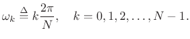 |
(10.11) |
Since the bandwidths, as defined, are
![\includegraphics[width=3in]{eps/sincbank}](http://www.dsprelated.com/josimages_new/sasp2/img1591.png)
System Diagram of the Running-Sum Filter Bank
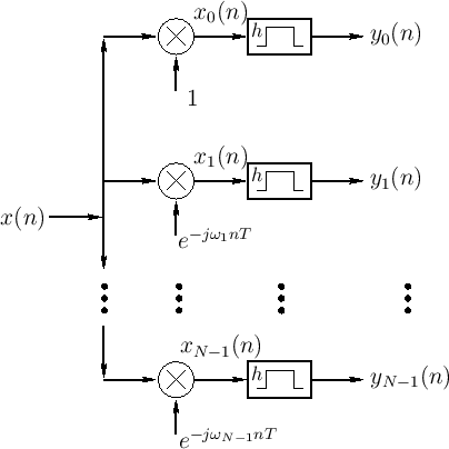
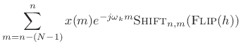
Figure 9.15 shows the system diagram of the complete ![]() -channel filter bank
constructed using length
-channel filter bank
constructed using length ![]() FIR running-sum lowpass filters. The
FIR running-sum lowpass filters. The
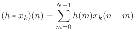
![]() th channel computes:
th channel computes:

DFT Filter Bank
Recall that the Length ![]() Discrete Fourier Transform (DFT) is
defined as
Discrete Fourier Transform (DFT) is
defined as
 |
(10.13) |
Comparing this to (9.12), we see that the filter-bank output
| (10.14) |
In other words, the filter-bank output at time
More generally, for all ![]() , we will call Fig.9.15 the DFT
filter bank. The DFT filter bank is the special case of the STFT for
which a rectangular window and hop size
, we will call Fig.9.15 the DFT
filter bank. The DFT filter bank is the special case of the STFT for
which a rectangular window and hop size ![]() are used.
are used.
The sliding DFT is obtained by advancing successive DFTs by one sample:
 |
(10.15) |
When
When ![]() is a power of 2, the DFT can be implemented using a Cooley-Tukey Fast
Fourier Transform (FFT) using only
is a power of 2, the DFT can be implemented using a Cooley-Tukey Fast
Fourier Transform (FFT) using only
![]() operations per
transform. By keeping track of the linear phase term (an
operations per
transform. By keeping track of the linear phase term (an
![]() modification), a DFT Filter Bank can be implemented efficiently using
an FFT. Uniform FIR filter banks are very often implemented in
practice using FFT software such as fftw.
modification), a DFT Filter Bank can be implemented efficiently using
an FFT. Uniform FIR filter banks are very often implemented in
practice using FFT software such as fftw.
Note that the channel bandwidths are narrow compared with half
the sampling rate (especially for large ![]() ), so that the filter bank
output signals
), so that the filter bank
output signals ![]() are oversampled, in general. We will
later look at downsampling the channel signals
are oversampled, in general. We will
later look at downsampling the channel signals ![]() to
obtain a ``hopping FFT'' filter bank. ``Sliding'' and ``hopping''
FFTs are special cases of the discrete-time Short Time Fourier
Transform (STFT). The STFT normally also uses a window
function other than the rectangular window used in this development
(the running-sum lowpass filter).
to
obtain a ``hopping FFT'' filter bank. ``Sliding'' and ``hopping''
FFTs are special cases of the discrete-time Short Time Fourier
Transform (STFT). The STFT normally also uses a window
function other than the rectangular window used in this development
(the running-sum lowpass filter).
Inverse DFT and the DFT Filter Bank Sum
The Length ![]() inverse DFT is given by [264]
inverse DFT is given by [264]
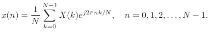 |
(10.16) |
This suggests that the DFT Filter Bank can be inverted by simply remodulating the baseband filter-bank signals
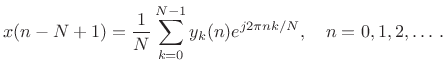 |
(10.17) |
This is in fact true, as we will later see. (It is straightforward to show as an exercise.)
Next Section:
FBS Window Constraints for R=1
Previous Section:
STFT Filter Bank


