


The Filter Bank Summation (FBS) Interpretation of the Short Time Fourier Transform (STFT)
Dual Views of the Short Time Fourier Transform (STFT)
In the overlap-add formulation of Chapter 8, we used a
hopping window to extract time-limited signals to which we
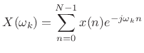
applied the DFT. Assuming for the moment that the hop size ![]() (the ``sliding DFT''), we have
(the ``sliding DFT''), we have
![$\displaystyle \zbox {X_m(\omega_k) = \sum_{n=-\infty}^\infty [w(n-m) x(n)] e^{-j\omega_k n}.} \protect$](http://www.dsprelated.com/josimages_new/sasp2/img1535.png)
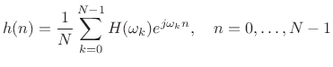
This is the usual definition of the Short-Time Fourier Transform (STFT) (§7.1). In this chapter, we will look at the STFT from two different points of view: the OverLap-Add (OLA) and Filter-Bank Summation (FBS) points of view. We will show that one is the Fourier dual of the other [9]. Next we will explore some implications of the filter-bank point of view and obtain some useful insights. Finally, some applications are considered.
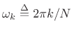
Overlap-Add (OLA) Interpretation of the STFT
In the OLA interpretation of the STFT, we apply a time-shifted window
![]() to our signal
to our signal ![]() , selecting data near time
, selecting data near time ![]() , and
compute the Fourier-transform to obtain the spectrum of the
, and
compute the Fourier-transform to obtain the spectrum of the ![]() th
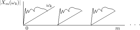
frame. As shown in Fig.9.1, the STFT is viewed as a
time-ordered sequence of spectra, one per frame, with the
frames overlapping in time.
th
frame. As shown in Fig.9.1, the STFT is viewed as a
time-ordered sequence of spectra, one per frame, with the
frames overlapping in time.
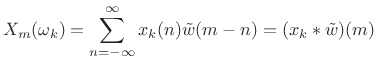
Filter-Bank Summation (FBS) Interpretation of the STFT
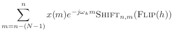
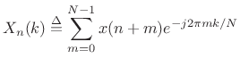
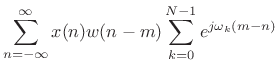
We can group the terms in the STFT definition differently to obtain
the filter-bank interpretation:
![$\displaystyle \sum_{n=-\infty}^\infty \underbrace{[ x(n)e^{-j\omega_k n}]}_{x_k(n)} w(n-m)$](http://www.dsprelated.com/josimages_new/sasp2/img1538.png)
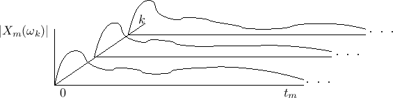
As will be explained further below (and illustrated further in Figures 9.3, 9.4, and 9.5), under the filter-bank interpretation, the spectrum of
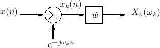
Expanding on the previous paragraph, the STFT (9.2) is computed by the following operations:
- Frequency-shift
 by
by  to get
 .
.
- Convolve
 with
with
 to get
 :
:
(10.3)
Note that the STFT analysis window ![]() is now interpreted as (the flip
of) a lowpass-filter impulse response. Since the analysis window
is now interpreted as (the flip
of) a lowpass-filter impulse response. Since the analysis window ![]() in the STFT is typically symmetric, we usually have
in the STFT is typically symmetric, we usually have
![]() .
This filter is effectively frequency-shifted to provide each channel
bandpass filter. If the cut-off frequency of the window transform is
.
This filter is effectively frequency-shifted to provide each channel
bandpass filter. If the cut-off frequency of the window transform is
![]() (typically half a main-lobe width), then each channel
signal can be downsampled significantly. This downsampling factor is
the FBS counterpart of the hop size
(typically half a main-lobe width), then each channel
signal can be downsampled significantly. This downsampling factor is
the FBS counterpart of the hop size ![]() in the OLA context.
in the OLA context.
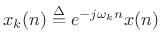
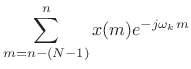
Figure 9.3 illustrates the filter-bank interpretation for ![]() (the ``sliding STFT''). The input signal
(the ``sliding STFT''). The input signal ![]() is frequency-shifted
by a different amount for each channel and lowpass filtered by the
(flipped) window.
is frequency-shifted
by a different amount for each channel and lowpass filtered by the
(flipped) window.
![\begin{psfrags}
% latex2html id marker 23871\psfrag{w}{\Large$\protect\hbox{\sc Flip}(w)$}\psfrag{x(n)}{\LARGE$x(n)$}\psfrag{X0}{\LARGE$X_n(\omega_{\scriptscriptstyle 0}$)}\psfrag{X1}{\LARGE$X_n(\omega_{\scriptscriptstyle 1}$)}\psfrag{XNm1}{\LARGE$X_n(\omega_{\scriptscriptstyle {N}-1})$}\psfrag{ejw0}{\huge$e^{-j\omega_{\scriptscriptstyle 0}n}$}\psfrag{ejw1}{\huge$e^{-j\omega_{\scriptscriptstyle 1}n}$}\psfrag{ejwNm1}{\huge$e^{-j\omega_{\scriptscriptstyle {N-1}}n}$}\psfrag{dR}{\LARGE$\downarrow R$}\psfrag{X}{\LARGE$\times$}\begin{figure}[htbp]
\includegraphics[width=3in]{eps/fbs1}
\caption{Sliding STFT analysis filter bank.
The $k$th channel of the filter bank computes
$X_n(\omega_k)=(x_k\ast \hbox{\sc Flip}{w})(n)$, where $x_k(n)\isdeftext
x(n)\exp(-j\omega_k n)$.
}
\end{figure}
\end{psfrags}](http://www.dsprelated.com/josimages_new/sasp2/img1552.png)
FBS and Perfect Reconstruction
An important property of the STFT established in Chapter 8 is that it is exactly invertible when the analysis window satisfies the constant-overlap-add constraint. That is, neglecting numerical round-off error, the inverse STFT reproduces the original input signal exactly. This is called the perfect reconstruction property of the STFT, and modern filter banks are usually designed with this property in mind [287].
In the OLA processors of Chapter 8, perfect reconstruction was
assured by using FFT analysis windows ![]() having the
Constant-Overlap-Add (COLA) property at the particular hop-size
having the
Constant-Overlap-Add (COLA) property at the particular hop-size
![]() used (see §8.2.1).
used (see §8.2.1).
In the Filter Bank Summation (FBS) interpretation of the STFT
(Eq.![]() (9.1)), it is the analysis filter-bank frequency
responses
(9.1)), it is the analysis filter-bank frequency
responses
![]() that are constrained to be COLA. We
will take a look at this more closely below.
that are constrained to be COLA. We
will take a look at this more closely below.
STFT Filter Bank
Each channel of an STFT filter bank implements the processing shown in
Fig.9.4. The same processing is shown in the frequency domain
in Fig.9.5. Note that the window transform ![]() is
complex-conjugated because the window
is
complex-conjugated because the window ![]() is flipped in the time
domain, i.e.,
is flipped in the time
domain, i.e.,
![]() when
when ![]() is real
[264].
is real
[264].
 |
These channels are then arranged in parallel to form a filter
bank, as shown in Fig.9.3. In practice, we need to know under
what conditions the channel filters ![]() will yield perfect
reconstruction when the channel signals are remodulated and summed.
(A sufficient condition for the sliding STFT is that the channel
frequency responses overlap-add to a constant over the unit circle in
the frequency domain.) Furthermore, since the channel signals are
heavily oversampled, particularly when the chosen window
will yield perfect
reconstruction when the channel signals are remodulated and summed.
(A sufficient condition for the sliding STFT is that the channel
frequency responses overlap-add to a constant over the unit circle in
the frequency domain.) Furthermore, since the channel signals are
heavily oversampled, particularly when the chosen window ![]() has low
side-lobe levels, we would like to be able to downsample the channel
signals without loss of information. It is indeed possible to
downsample the channel signals while retaining the perfect
reconstruction property, as we will see in §9.8.1.
has low
side-lobe levels, we would like to be able to downsample the channel
signals without loss of information. It is indeed possible to
downsample the channel signals while retaining the perfect
reconstruction property, as we will see in §9.8.1.
Computational Examples in Matlab
In this section, we will take a look at some STFT filter-bank output signals when the input signal is a ``chirp.'' A chirp signal is generally defined as a sinusoid having a linearly changing frequency over time:
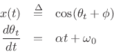
The matlab code is as follows:
N=10;           % number of filters = DFT length
fs=1000;        % sampling frequency (arbitrary)
D=1;            % duration in seconds

L = ceil(fs*D)+1; % signal duration (samples)
n = 0:L-1;        % discrete-time axis (samples)
t = n/fs;         % discrete-time axis (sec)
x = chirp(t,0,D,fs/2);   % sine sweep from 0 Hz to fs/2 Hz
%x = echirp(t,0,D,fs/2); % for complex "analytic" chirp
x = x(1:L);       % trim trailing zeros at end
h = ones(1,N);    % Simple DFT lowpass = rectangular window
%h = hamming(N);  % Better DFT lowpass = Hamming window
X = zeros(N,L);   % X will be the filter bank output
for k=1:N         % Loop over channels
  wk = 2*pi*(k-1)/N;
  xk = exp(-j*wk*n).* x;  % Modulation by complex exponential
  X(k,:) = filter(h,1,xk);
end
Figure 9.6 shows the input and output-signal real parts for a ten-channel DFT filter bank based on the rectangular window as derived above. The imaginary parts of the channel-filter output signals are similar so they're not shown. Notice how the amplitude envelope in each channel follows closely the amplitude response of the running-sum lowpass filter. This is more clearly seen when the absolute values of the output signals are viewed, as shown in Fig.9.7.
![\includegraphics[width=\twidth,height=6.5in]{eps/dcrrrp}](http://www.dsprelated.com/josimages_new/sasp2/img1560.png) |
![\includegraphics[width=\twidth,height=6.5in]{eps/dcrr}](http://www.dsprelated.com/josimages_new/sasp2/img1561.png) |
Replacing the rectangular window with the Hamming window gives much improved channel isolation at the cost of doubling the channel bandwidth, as shown in Fig.9.8. Now the window-transform side lobes (lowpass filter stop-band response) are not really visible to the eye. The intense ``beating'' near dc and half the sampling rate is caused by the fact that we used a real chirp. The matlab for this chirp boils down to the following:
function x = chirp(t,f0,t1,f1);
beta = (f1-f0)./t1;
x = cos(2*pi * ( 0.5* beta .* (t.^2) + f0*t));
We can replace this real chirp with a complex ``analytic'' chirp by replacing the last line above by the following:
x = exp(j*(2*pi * ( 0.5* beta .* (t.^2) + f0*t)));Since the analytic chirp does not contain a negative-frequency component which beats with the positive-frequency component, we obtain the cleaner looking output moduli shown in Fig.9.9.
Since our chirp frequency goes from zero to half the sampling rate, we
are no longer exciting the negative-frequency channels. (To fully
traverse the frequency axis with a complex chirp, we would need to
sweep it from ![]() to
to ![]() .) We see in Fig.9.9 that there is
indeed relatively little response in the ``negative-frequency
channels'' for which
.) We see in Fig.9.9 that there is
indeed relatively little response in the ``negative-frequency
channels'' for which ![]() , but there is some noticeable
``leakage'' from channel 0 into channel
, but there is some noticeable
``leakage'' from channel 0 into channel ![]() , and channel 5 similarly
leaks into channel 6. Since the channel pass-bands overlap
approximately 75%, this is not unexpected. The automatic vertical
scaling in the channel 7 and 8 plots shows clearly the side-lobe
structure of the Hamming window. Finally, notice also that the length
, and channel 5 similarly
leaks into channel 6. Since the channel pass-bands overlap
approximately 75%, this is not unexpected. The automatic vertical
scaling in the channel 7 and 8 plots shows clearly the side-lobe
structure of the Hamming window. Finally, notice also that the length
![]() start-up transient is visible in each channel output just
after time 0.
start-up transient is visible in each channel output just
after time 0.
![\includegraphics[width=\twidth,height=6.5in]{eps/dcrh}](http://www.dsprelated.com/josimages_new/sasp2/img1565.png) |
![\includegraphics[width=\twidth,height=6.5in]{eps/dacrh}](http://www.dsprelated.com/josimages_new/sasp2/img1566.png) |
The DFT Filter Bank
To obtain insight into the operation of filter banks implemented using an FFT, this section will derive the details of the DFT Filter Bank. More general STFT filter banks are obtained by using different windows and hop sizes, but otherwise are no different from the basic DFT filter bank.
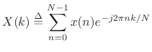
The Discrete Fourier Transform (DFT) is defined by [264]
 |
(10.4) |
where
 . In this section, we will show how the DFT can be computed
exactly from a bank of
. In this section, we will show how the DFT can be computed
exactly from a bank of
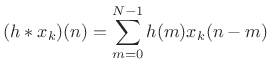
The Running-Sum Lowpass Filter
Perhaps the simplest FIR lowpass filter is the so-called
running-sum lowpass filter [175]. The impulse
response of the length ![]() running-sum lowpass filter is given by
running-sum lowpass filter is given by
![$\displaystyle h(n) \isdef \left\{\begin{array}{ll} 1, & n=0,1,2,...,N-1 \\ [5pt] 0, & \hbox{otherwise.} \\ \end{array} \right. \protect$](http://www.dsprelated.com/josimages_new/sasp2/img1568.png)
Figure 9.10 depicts the generic operation of filtering ![]() by
by ![]() to produce
to produce ![]() , where
, where ![]() is the impulse response of the
filter. The output signal is given by the convolution of
is the impulse response of the
filter. The output signal is given by the convolution of ![]() and
and ![]() :
:
In this form, it is clear why the filter (9.5) is called
``running sum'' filter. Dividing it by ![]() , it becomes a ``moving
average'' filter, averaging the most recent
, it becomes a ``moving
average'' filter, averaging the most recent ![]() input samples.
input samples.
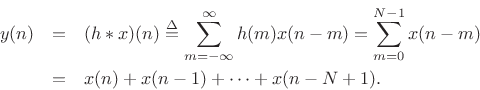
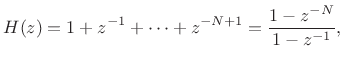
The transfer function of the running-sum filter is given by [263]
 |
(10.6) |
so that its frequency response is
![\begin{eqnarray*}
H(e^{j\omega}) &=& \frac{1-e^{-j\omega N}}{1-e^{-j\omega }}
= \frac{e^{-j\omega N/2}}{e^{-j\omega /2}}
\frac{\sin(\omega N/2)}{\sin(\omega /2)}\\ [10pt]
&\isdef &
Ne^{-j\omega(N-1)/2} \hbox{asinc}_N(\omega ).
\end{eqnarray*}](http://www.dsprelated.com/josimages_new/sasp2/img1572.png)
Recall that the term
![]() is a linear phase
term corresponding to a delay of
is a linear phase
term corresponding to a delay of ![]() samples (half of the FIR
filter order). This arises because we defined the running-sum lowpass
filter as a causal, linear phase filter.
samples (half of the FIR
filter order). This arises because we defined the running-sum lowpass
filter as a causal, linear phase filter.
We encountered the ``aliased sinc function''
 |
(10.7) |
previously in Chapter 5 (§3.1.2) and elsewhere as the Fourier transform (DTFT) of a sampled rectangular pulse (or rectangular window).
Note that the dc gain of the length ![]() running sum filter is
running sum filter is ![]() . We
could use a moving average instead of a running sum (
. We
could use a moving average instead of a running sum (
![]() ) to obtain unity dc gain.
) to obtain unity dc gain.
![\includegraphics[width=4in]{eps/sincabs}](http://www.dsprelated.com/josimages_new/sasp2/img1577.png)
Figure 9.11 shows the amplitude response of the running-sum
lowpass filter for length ![]() . The gain at dc is
. The gain at dc is ![]() , and nulls
occur at
, and nulls
occur at
![]() and
and ![]() . These nulls occur
at the sinusoidal frequencies having respectively one and two periods
under the 5-sample ``rectangular window''. (Three periods would need
at least
. These nulls occur
at the sinusoidal frequencies having respectively one and two periods
under the 5-sample ``rectangular window''. (Three periods would need
at least
![]() samples, so
samples, so ![]() doesn't ``fit''.) Since
the pass-band about dc is not flat, it is better to call this a
``dc-pass filter'' rather than a ``lowpass filter.'' We could also
call it a dc sampling filter.10.1
doesn't ``fit''.) Since
the pass-band about dc is not flat, it is better to call this a
``dc-pass filter'' rather than a ``lowpass filter.'' We could also
call it a dc sampling filter.10.1
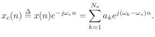
Modulation by a Complex Sinusoid
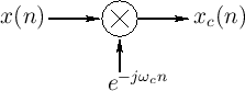
Figure 9.12 shows the system diagram for complex
demodulation.10.2The input signal ![]() is multiplied by a
complex sinusoid to produce the frequency-shifted result
is multiplied by a
complex sinusoid to produce the frequency-shifted result
| (10.8) |
Given a signal expressed as a sum of sinusoids,
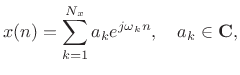 |
(10.9) |
then the demodulation produces
 |
(10.10) |
We see that frequency
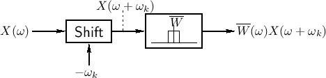
Making a Bandpass Filter from a Lowpass Filter
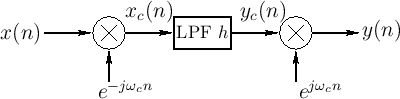 |
Figure 9.13 shows how a bandpass filter can be made using a lowpass
filter together with modulation. The input spectrum is
frequency-shifted by ![]() , lowpass filtered, then
frequency-shifted by
, lowpass filtered, then
frequency-shifted by ![]() , thereby creating a bandpass filter
centered at frequency
, thereby creating a bandpass filter
centered at frequency ![]() . From our experience with
rectangular-window transforms (Fig.9.11 being one example), we
can say that the bandpass-filter bandwidth is equal to the main-lobe
width of the aliased sinc function, or
. From our experience with
rectangular-window transforms (Fig.9.11 being one example), we
can say that the bandpass-filter bandwidth is equal to the main-lobe
width of the aliased sinc function, or ![]() radians per sample
(measured from zero-crossing to zero-crossing).
radians per sample
(measured from zero-crossing to zero-crossing).
Uniform Running-Sum Filter Banks
Using a length ![]() running-sum filter, let's make
running-sum filter, let's make ![]() bandpass filters
tuned to center frequencies
bandpass filters
tuned to center frequencies
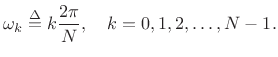 |
(10.11) |
Since the bandwidths, as defined, are
![\includegraphics[width=3in]{eps/sincbank}](http://www.dsprelated.com/josimages_new/sasp2/img1591.png)
System Diagram of the Running-Sum Filter Bank
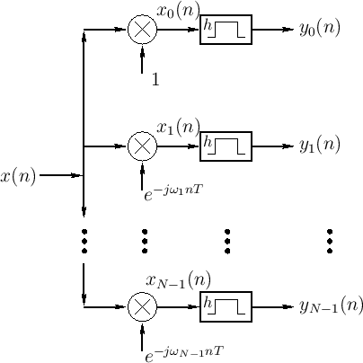
Figure 9.15 shows the system diagram of the complete ![]() -channel filter bank
constructed using length
-channel filter bank
constructed using length ![]() FIR running-sum lowpass filters. The
FIR running-sum lowpass filters. The
![]() th channel computes:
th channel computes:

DFT Filter Bank
Recall that the Length ![]() Discrete Fourier Transform (DFT) is
defined as
Discrete Fourier Transform (DFT) is
defined as
 |
(10.13) |
Comparing this to (9.12), we see that the filter-bank output
| (10.14) |
In other words, the filter-bank output at time
More generally, for all ![]() , we will call Fig.9.15 the DFT
filter bank. The DFT filter bank is the special case of the STFT for
which a rectangular window and hop size
, we will call Fig.9.15 the DFT
filter bank. The DFT filter bank is the special case of the STFT for
which a rectangular window and hop size ![]() are used.
are used.
The sliding DFT is obtained by advancing successive DFTs by one sample:
 |
(10.15) |
When
When ![]() is a power of 2, the DFT can be implemented using a Cooley-Tukey Fast
Fourier Transform (FFT) using only
is a power of 2, the DFT can be implemented using a Cooley-Tukey Fast
Fourier Transform (FFT) using only
![]() operations per
transform. By keeping track of the linear phase term (an
operations per
transform. By keeping track of the linear phase term (an
![]() modification), a DFT Filter Bank can be implemented efficiently using
an FFT. Uniform FIR filter banks are very often implemented in
practice using FFT software such as fftw.
modification), a DFT Filter Bank can be implemented efficiently using
an FFT. Uniform FIR filter banks are very often implemented in
practice using FFT software such as fftw.
Note that the channel bandwidths are narrow compared with half
the sampling rate (especially for large ![]() ), so that the filter bank
output signals
), so that the filter bank
output signals ![]() are oversampled, in general. We will
later look at downsampling the channel signals
are oversampled, in general. We will
later look at downsampling the channel signals ![]() to
obtain a ``hopping FFT'' filter bank. ``Sliding'' and ``hopping''
FFTs are special cases of the discrete-time Short Time Fourier
Transform (STFT). The STFT normally also uses a window
function other than the rectangular window used in this development
(the running-sum lowpass filter).
to
obtain a ``hopping FFT'' filter bank. ``Sliding'' and ``hopping''
FFTs are special cases of the discrete-time Short Time Fourier
Transform (STFT). The STFT normally also uses a window
function other than the rectangular window used in this development
(the running-sum lowpass filter).
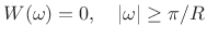
Inverse DFT and the DFT Filter Bank Sum
The Length ![]() inverse DFT is given by [264]
inverse DFT is given by [264]
 |
(10.16) |
This suggests that the DFT Filter Bank can be inverted by simply remodulating the baseband filter-bank signals
 |
(10.17) |
This is in fact true, as we will later see. (It is straightforward to show as an exercise.)
FBS Window Constraints for R=1
Recall that in overlap-add (Chapter 8), perfect
reconstruction required only that the analysis window ![]() meet a
constant overlap-add (COLA) constraint:
meet a
constant overlap-add (COLA) constraint:
 |
(10.18) |
where
The Filter Bank Summation (FBS) is interpreted as a demodulation
(frequency shift by ![]() ) and subsequent lowpass filtering by
) and subsequent lowpass filtering by
![]() . Therefore, to
resynthesize our original signal, we need to remodulate each
baseband signal and sum up the channels. For
. Therefore, to
resynthesize our original signal, we need to remodulate each
baseband signal and sum up the channels. For ![]() (no
downsampling), this sum is given by [9]
(no
downsampling), this sum is given by [9]
![$\displaystyle \sum_{k=0}^{N-1} \left[ \sum_{n=-\infty}^\infty
x(n)w(n-m)e^{-j\omega_kn} \right] e^{j\omega_km}$](http://www.dsprelated.com/josimages_new/sasp2/img1614.png)
We have thus derived the following sufficient condition for perfect reconstruction [213]:
Since normally our windows are shorter than
Nyquist(N) Windows
In (9.19) of the previous section, we derived that the FBS reconstruction sum gives
 |
(10.20) |
where
| (10.21) |
This is simply a gain term, and so we are able to recover the original signal exactly. (Zero-phase windows are appropriate here.)
If the window length is larger than the number of analysis frequencies
(![]() ), we can still obtain perfect reconstruction provided
), we can still obtain perfect reconstruction provided
| (10.22) |
When this holds, we say the window is
![\includegraphics[width=\twidth]{eps/colawin}](http://www.dsprelated.com/josimages_new/sasp2/img1628.png)
Duality of COLA and Nyquist Conditions
Let
![]() denote constant overlap-add using hop size
denote constant overlap-add using hop size ![]() . Then we
have (by the Poisson summation formula Eq.
. Then we
have (by the Poisson summation formula Eq.![]() (8.30))
(8.30))
![\begin{eqnarray*}
w &\in& \hbox{\sc Nyquist}(N) \Leftrightarrow W \in \hbox{\sc Cola}(2\pi/N) \qquad \hbox{(FBS)} \\ [10pt]
w &\in& \hbox{\sc Cola}(R) \Leftrightarrow W \in \hbox{\sc Nyquist}(2\pi/R) \qquad \hbox{(OLA)}
\end{eqnarray*}](http://www.dsprelated.com/josimages_new/sasp2/img1630.png)
Specific Windows
- Recall that the rectangular window transform is
 , implying the rectangular window itself is
 ,
which is obvious.
,
which is obvious.
- The window transform for the Hamming family is
 ,
implying that Hamming windows are
,
implying that Hamming windows are
 , which we also knew.
- The rectangular window transform is also
 for any integer
 , implying that all hop sizes given
by
, implying that all hop sizes given
by  for
for
 are COLA.
- Because its side lobes are the same width as the sinc side lobes,
the Hamming window transform is also
,for any integer
 , implying hop sizes
are good, for
, implying hop sizes
are good, for
 . Thus, the available hop sizes for the Hamming
window family include all of those for the rectangular window
except one (
. Thus, the available hop sizes for the Hamming
window family include all of those for the rectangular window
except one ( ).
).
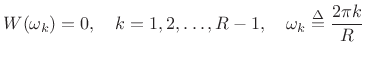
The Nyquist Property on the Unit Circle
As a degenerate case, note that ![]() is COLA for any window, while no
window transform is
is COLA for any window, while no
window transform is
![]() except the zero window. (since it
would have to be zero at dc, and we do not consider such windows).
Did the theory break down for
except the zero window. (since it
would have to be zero at dc, and we do not consider such windows).
Did the theory break down for ![]() ?
?
Intuitively, the
![]() condition on the window transform
condition on the window transform
![]() ensures that all nonzero multiples of the
time-domain-frame-rate
ensures that all nonzero multiples of the
time-domain-frame-rate ![]() will be zeroed out over the interval
will be zeroed out over the interval
![]() along the frequency axis. When the frame-rate equals the
sampling rate (
along the frequency axis. When the frame-rate equals the
sampling rate (![]() ), there are no frame-rate multiples in the
range
), there are no frame-rate multiples in the
range
![]() . (The range
. (The range ![]() gives the same result.)
When
gives the same result.)
When ![]() , there is exactly one frame-rate multiple at
, there is exactly one frame-rate multiple at ![]() . When
. When
![]() , there are two at
, there are two at
![]() . When
. When ![]() , they are at
, they are at ![]() and
and ![]() , and so on.
, and so on.
We can cleanly handle the special case of ![]() by defining all
functions over the unit circle as being
by defining all
functions over the unit circle as being
![]() when there are no
frame-rate multiples in the range
when there are no
frame-rate multiples in the range
![]() . Thus, a discrete-time
spectrum
. Thus, a discrete-time
spectrum
![]() is said to be
is said to be
![]() if
if
![]() , for all
, for all
![]() , where
, where
![]() (the ``floor function'') denotes the greatest integer less
than or equal to
(the ``floor function'') denotes the greatest integer less
than or equal to ![]() .
.
Portnoff Windows
In 1976 [212], Portnoff observed that any window ![]() of the form
of the form
| (10.23) |
being
sinc |
(10.24) |
(the unit-amplitude sinc function with zeros at all nonzero integers).
Portnoff suggested that, in practical usage, windowed data segments
longer than the FFT size should be time-aliased about length
![]() prior to performing an FFT. This result is readily derived from the
definition of the time-normalized STFT introduced in Eq.
prior to performing an FFT. This result is readily derived from the
definition of the time-normalized STFT introduced in Eq.![]() (8.21):
(8.21):
![\begin{eqnarray*}
{\tilde X}_m(\omega_k)
&\isdef & \hbox{\sc Sample}_{\Omega_N,k}\left(\hbox{\sc DTFT}\left({\tilde x}_m\right)\right) \\
&\isdef & \hbox{\sc Sample}_{\Omega_N,k}\left(\hbox{\sc DTFT}\left(\hbox{\sc Shift}_{-m}(x)\cdot w\right)\right) \\
&=& \sum_{n=-\infty}^\infty x(n+m)w(n)e^{-j\omega_k n}\quad\hbox{(now let $n\isdef lN+i$)}\\
&=& \sum_{l=-\infty}^\infty \sum_{i=0}^{N-1}x(lN+i+m)w(lN+i)
\underbrace{e^{-j\omega_k (lN+i)}}_{e^{-j\omega_k i}}\\
&=& \sum_{i=0}^{N-1}\left[\sum_{l=-\infty}^\infty x(lN+i+m)w(lN+i)\right]
e^{-j\omega_k i}\\
&=& \sum_{i=0}^{N-1}\hbox{\sc Alias}_{N,i}[\hbox{\sc Shift}_{-m}(x)\cdot w] e^{-j\omega_k i}\\
&\isdef & \hbox{\sc DFT}_{N,k}\{\hbox{\sc Alias}_N[\hbox{\sc Shift}_{-m}(x)\cdot w]\},
\end{eqnarray*}](http://www.dsprelated.com/josimages_new/sasp2/img1655.png)
where
 as usual.
Choosing ![]() allows multiple side lobes of the sinc function to
alias in on the main lobe. This gives channel filters in the
frequency domain which are sharper bandpass filters while remaining COLA.
I.e., there is less channel cross-talk in the frequency domain.
However, the time-aliasing
corresponds to undersampling in the frequency domain, implying less
robustness to spectral modifications, since such modifications can
disturb the time-domain aliasing cancellation. Since the hop size
needs to be less than
allows multiple side lobes of the sinc function to
alias in on the main lobe. This gives channel filters in the
frequency domain which are sharper bandpass filters while remaining COLA.
I.e., there is less channel cross-talk in the frequency domain.
However, the time-aliasing
corresponds to undersampling in the frequency domain, implying less
robustness to spectral modifications, since such modifications can
disturb the time-domain aliasing cancellation. Since the hop size
needs to be less than ![]() , the overall filter bank based on a Portnoff
window remains oversampled in the time domain.
, the overall filter bank based on a Portnoff
window remains oversampled in the time domain.
Downsampled STFT Filter Banks
We now look at STFT filter banks which are downsampled by the
factor ![]() . The downsampling factor
. The downsampling factor ![]() corresponds to a hop size
of
corresponds to a hop size
of ![]() samples in the overlap-add view of the STFT. From the
filter-bank point of view, the impact of
samples in the overlap-add view of the STFT. From the
filter-bank point of view, the impact of ![]() is aliasing in
the channel signals when the lowpass filter (analysis window) is less
than ideal. When the conditions for perfect reconstruction are met,
this aliasing will be canceled in the reconstruction (when
the filter-bank channel signals are remodulated and summed).
is aliasing in
the channel signals when the lowpass filter (analysis window) is less
than ideal. When the conditions for perfect reconstruction are met,
this aliasing will be canceled in the reconstruction (when
the filter-bank channel signals are remodulated and summed).
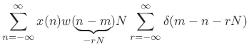
Downsampled STFT Filter Bank
So far we have considered only ![]() (the ``sliding'' DFT) in our
filter-bank interpretation of the STFT. For
(the ``sliding'' DFT) in our
filter-bank interpretation of the STFT. For ![]() we obtain a
downsampled version of
we obtain a
downsampled version of
![]() :
:
![\begin{eqnarray*}
X_{mR}(\omega_k) &=& \sum_{n=-\infty}^\infty [x(n)e^{-j\omega_kn}]\tilde{w}(mR-n)
\hspace{1.2cm} (\tilde{w} \mathrel{\stackrel{\Delta}{=}}\hbox{\sc Flip}(w)) \\
&=& (x_k \ast {\tilde w})(mR)
\end{eqnarray*}](http://www.dsprelated.com/josimages_new/sasp2/img1659.png)
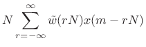
Let us define the downsampled time index as
![]() so
that
so
that
![$\displaystyle X_{\tilde{m}}(\omega_k) = \sum_{n=-\infty}^\infty [x(n)e^{-j\omega_kn}]\tilde{w}(\tilde{m}-n) \mathrel{\stackrel{\Delta}{=}}\left(x_k \ast {\tilde w}\right)(\tilde{m})$](http://www.dsprelated.com/josimages_new/sasp2/img1661.png) |
(10.25) |
i.e.,
![\begin{psfrags}
% latex2html id marker 25320\psfrag{w}{{\Large $\protect\hbox{\sc Flip}(w)$\ }}\psfrag{x(n)}{\Large $x(n)$\ }\psfrag{Xm}{\Large $X_m$\ }\psfrag{Xmt}{\Large $X_{\tilde{m}}$\ }\psfrag{X0}{\Large $X_{\tilde{m}}(\omega_0)$\ }\psfrag{X1}{\Large $X_{\tilde{m}}(\omega_1)$\ }\psfrag{XNm1}{\Large $X_{\tilde{m}}(\omega_{N-1})$\ }\psfrag{ejw0}{\Large $e^{-j\omega_0n}$\ }\psfrag{ejw1}{\Large $e^{-j\omega_1n}$\ }\psfrag{ejwNm1}{\Large $e^{-j\omega_{N-1}n}$\ }\psfrag{dR}{\Large $\downarrow R$\ }\begin{figure}[htbp]
\includegraphics[width=\twidth]{eps/fbs2}
\caption{Downsampled STFT filter bank.}
\end{figure}
\end{psfrags}](http://www.dsprelated.com/josimages_new/sasp2/img1665.png)
Note that this can be considered an implementation of a phase vocoder filter bank [212]. (See §G.5 for an introduction to the vocoder.)
Filter Bank Reconstruction
![\begin{psfrags}
% latex2html id marker 25351\psfrag{w}{{\Large $f$\ }} % should fix source (.draw file)\begin{figure}[htbp]
\includegraphics[width=\twidth]{eps/FBSreconstruct}
\caption{Interpolated, remodulated, filter-bank sum.}
\end{figure}
\end{psfrags}](http://www.dsprelated.com/josimages_new/sasp2/img1666.png)
Since the channel signals are downsampled, we generally need
interpolation in the reconstruction. Figure 9.18
indicates how we might pursue this. From studying the overlap-add
framework, we know that the inverse STFT is exact when the
window ![]() is
is
![]() , that is, when
, that is, when
![]() is constant.
In only these cases can the STFT be considered a perfect
reconstruction filter bank. From the Poisson Summation Formula in
§8.3.1, we know that a condition
equivalent to the COLA condition is that the window
transform
is constant.
In only these cases can the STFT be considered a perfect
reconstruction filter bank. From the Poisson Summation Formula in
§8.3.1, we know that a condition
equivalent to the COLA condition is that the window
transform ![]() have notches at all harmonics
of the frame rate, i.e.,
have notches at all harmonics
of the frame rate, i.e.,
![]() for
for
![]() . In the
present context (filter-bank point of view), perfect reconstruction
appears impossible for
. In the
present context (filter-bank point of view), perfect reconstruction
appears impossible for ![]() , because for ideal reconstruction
after downsampling, the channel anti-aliasing filter (
, because for ideal reconstruction
after downsampling, the channel anti-aliasing filter (![]() ) and
interpolation filter (
) and
interpolation filter (![]() ) have to be ideal lowpass filters.
This is a true conclusion in any single channel, but not for the
filter bank as a whole. We know, for example, from the overlap-add
interpretation of the STFT that perfect reconstruction occurs for
hop-sizes greater than 1 as long as the COLA condition is met. This
is an interesting paradox to which we will return shortly.
) have to be ideal lowpass filters.
This is a true conclusion in any single channel, but not for the
filter bank as a whole. We know, for example, from the overlap-add
interpretation of the STFT that perfect reconstruction occurs for
hop-sizes greater than 1 as long as the COLA condition is met. This
is an interesting paradox to which we will return shortly.
What we would expect in the filter-bank context is that the
reconstruction can be made arbitrarily accurate given better and
better lowpass filters ![]() and
and ![]() which cut off at
which cut off at
![]() (the folding frequency associated with down-sampling by
(the folding frequency associated with down-sampling by ![]() ). This is
the right way to think about the STFT when spectral
modifications are involved.
). This is
the right way to think about the STFT when spectral
modifications are involved.
In Chapter 11 we will develop the general topic of perfect reconstruction filter banks, and derive various STFT processors as special cases.
Downsampling with Anti-Aliasing
![\includegraphics[width=3in]{eps/FBSonechan}](http://www.dsprelated.com/josimages_new/sasp2/img1671.png)
In OLA, the hop size ![]() is governed by the COLA constraint
is governed by the COLA constraint
 |
(10.26) |
In FBS,
![\includegraphics[width=3in]{eps/IdealWindowFD}](http://www.dsprelated.com/josimages_new/sasp2/img1674.png)
Properly Anti-Aliasing Window Transforms
For simplicity, define window-transform bandlimits at first
zero-crossings about the main lobe. Given the first zero of
![]() at
at
![]() , we obtain
, we obtain
 |
(10.27) |
The following table gives maximum hop sizes for various window types in the Blackman-Harris family, where
| L | Window Type (Length |
|
|
| 1 | Rectangular | M/2 | M |
| 2 | Generalized Hamming | M/4 | M/2 |
| 3 | Blackman Family | M/6 | M/3 |
| L | M/2L | M/L |
It is interesting to note that the maximum COLA hop size is
double the maximum downsampling factor which avoids aliasing of the
main lobe of the window transform in FFT-bin signals
![]() . Since the COLA constraint is a sufficient condition
for perfect reconstruction, this aliasing is quite heavy (see
Fig.9.21), yet it is all canceled in the
reconstruction. The general theory of aliasing cancellation in perfect
reconstruction filter banks will be taken up in Chapter 11.
. Since the COLA constraint is a sufficient condition
for perfect reconstruction, this aliasing is quite heavy (see
Fig.9.21), yet it is all canceled in the
reconstruction. The general theory of aliasing cancellation in perfect
reconstruction filter banks will be taken up in Chapter 11.
![\includegraphics[width=3in]{eps/WindowAliasingFD}](http://www.dsprelated.com/josimages_new/sasp2/img1681.png)
It is important to realize that aliasing cancellation is
disturbed by FBS spectral modifications.10.4For robustness in the presence of spectral modifications, it is
advisable to keep
![]() . For compression, it
is common to use
. For compression, it
is common to use
![]() together with a ``synthesis window'' in a weighted overlap-add (WOLA)
scheme (§8.6).
together with a ``synthesis window'' in a weighted overlap-add (WOLA)
scheme (§8.6).
Hop Sizes for WOLA
In the weighted overlap-add method, with the synthesis (output) window equal to the analysis (input) window, we have the following modification of the recommended maximum hop-size table:
| L | In and Out Window (Length |
|
|
| 1 | Rectangular ( |
M/2 | M |
| 2 | Generalized Hamming ( |
M/6 | M/3 |
| 3 | Blackman Family ( |
M/10 | M/5 |
| L | M/(4L-2) | M/(2L-1) |
-
 is equal to
  divided by the main-lobe width
in ``side lobes'', while
divided by the main-lobe width
in ``side lobes'', while
-
 is
divided by the first notch
frequency in the window transform (lowest available frame rate at
which all frame-rate harmonics are notched).
is
divided by the first notch
frequency in the window transform (lowest available frame rate at
which all frame-rate harmonics are notched).
- For windows in the Blackman-Harris families, and
with main-lobe widths defined from zero-crossing to zero-crossing,
 .
.
Constant-Overlap-Add (COLA) Cases
- Weak COLA: Window transform has zeros at frame-rate harmonics:
- Perfect OLA reconstruction
- Relies on aliasing cancellation in frequency domain
- Aliasing cancellation is disturbed by spectral modifications
- See Portnoff for further details
- Strong COLA: Window transform is bandlimited consistent with
downsampling by the frame rate:
- Perfect OLA reconstruction
- No aliasing
- better for spectral modifications
- Time-domain window infinitely long in ideal case
Hamming Overlap-Add Example
Matlab code:
M = 33;         % window length
w = hamming(M);
R = (M-1)/2;    % maximum hop size
w(M) = 0;       % 'periodic Hamming' (for COLA)
%w(M) = w(M)/2; % another solution,
%w(1) = w(1)/2; %  interesting to compare
![\includegraphics[width=\textwidth ]{eps/olaHammingC}](http://www.dsprelated.com/josimages_new/sasp2/img1687.png)
Periodic-Hamming OLA from Poisson Summation Formula
Matlab code:
ff = 1/R; % frame rate (fs=1)
N = 6*M;  % no. samples to look at OLA
sp = ones(N,1)*sum(w)/R; % dc term (COLA term)
ubound = sp(1);  % try easy-to-compute upper bound
lbound = ubound; % and lower bound
n = (0:N-1)';
for (k=1:R-1) % traverse frame-rate harmonics
  f=ff*k;
  csin = exp(j*2*pi*f*n); % frame-rate harmonic
  % find exact window transform at frequency f
  Wf = w' * conj(csin(1:M));
  hum = Wf*csin;   % contribution to OLA "hum"
  sp = sp + hum/R; % "Poisson summation" into OLA
  % Update lower and upper bounds:
  Wfb = abs(Wf);
  ubound = ubound + Wfb/R; % build upper bound
  lbound = lbound - Wfb/R; % build lower bound
end
In this example, the overlap-add is theoretically a perfect constant
(equal to ![]() ) because the frame rate and all its harmonics
coincide with nulls in the window transform (see
Fig.9.24). A plot of the steady-state
overlap-add and that computed using the Poisson Summation Formula (not
shown) is constant to within numerical precision. The
difference between the actual overlap-add and that computed
using the PSF is shown in Fig.9.23. We verify that the
difference is on the order of
) because the frame rate and all its harmonics
coincide with nulls in the window transform (see
Fig.9.24). A plot of the steady-state
overlap-add and that computed using the Poisson Summation Formula (not
shown) is constant to within numerical precision. The
difference between the actual overlap-add and that computed
using the PSF is shown in Fig.9.23. We verify that the
difference is on the order of ![]() , which is close enough to
zero in double-precision (64-bit) floating-point computations. We
thus verify that the overlap-add of a length
, which is close enough to
zero in double-precision (64-bit) floating-point computations. We
thus verify that the overlap-add of a length ![]() Hamming window using
a hop size of
Hamming window using
a hop size of
![]() samples is constant to within machine
precision.
samples is constant to within machine
precision.
![\includegraphics[width=\textwidth ]{eps/olassmmpHammingC}](http://www.dsprelated.com/josimages_new/sasp2/img1692.png)
Figure 9.24 shows the zero-padded DFT of the
modified Hamming window we're using (
![]() ) with the
frame-rate harmonics marked. In this example (
) with the
frame-rate harmonics marked. In this example (![]() ), the upper
half of the main lobe aliases into the lower half of the main
lobe. (In fact, all energy above the folding frequency
), the upper
half of the main lobe aliases into the lower half of the main
lobe. (In fact, all energy above the folding frequency ![]() aliases into the lower half of the main lobe.) While this window and
hop size still give perfect reconstruction under the STFT, spectral
modifications will disturb the aliasing cancellation during
reconstruction. This ``undersampled'' configuration is suitable as a
basis for compression applications.
aliases into the lower half of the main lobe.) While this window and
hop size still give perfect reconstruction under the STFT, spectral
modifications will disturb the aliasing cancellation during
reconstruction. This ``undersampled'' configuration is suitable as a
basis for compression applications.
![\includegraphics[width=\textwidth ]{eps/windowTransformHammingC}](http://www.dsprelated.com/josimages_new/sasp2/img1695.png)
Note that if we were to cut ![]() in half to
in half to ![]() , then the folding
frequency in Fig.9.24 would coincide with the
first null in the window transform. Since the frame rate and all its
harmonics continue to land on nulls in the window transform,
overlap-add is still exact. At this reduced hop size, however, the
STFT becomes much more robust to spectral modifications, because all
aliasing in the effective downsampled filter bank is now weighted by
the side lobes of the window transform, with no aliasing
components coming from within the main lobe. This is the central
result of [9].
, then the folding
frequency in Fig.9.24 would coincide with the
first null in the window transform. Since the frame rate and all its
harmonics continue to land on nulls in the window transform,
overlap-add is still exact. At this reduced hop size, however, the
STFT becomes much more robust to spectral modifications, because all
aliasing in the effective downsampled filter bank is now weighted by
the side lobes of the window transform, with no aliasing
components coming from within the main lobe. This is the central
result of [9].
Kaiser Overlap-Add Example
Matlab code:
M = 33;    % Window length
beta = 8;
w = kaiser(M,beta);
R = floor(1.7*(M-1)/(beta+1)); % ROUGH estimate (gives R=6)
Figure 9.25 plots the overlap-added Kaiser windows, and Fig.9.26 shows the steady-state overlap-add (a time segment sometime after the first 30 samples). The ``predicted'' OLA is computed using the Poisson Summation Formula using the same matlab code as before. Note that the Poisson summation formula gives exact results to within numerical precision. The upper (lower) bound was computed by summing (subtracting) the window-transform magnitudes at all frame-rate harmonics to (from) the dc gain of the window. This is one example of how the PSF can be used to estimate upper and lower bounds on OLA error.
![\includegraphics[width=\textwidth ]{eps/olakaiserC}](http://www.dsprelated.com/josimages_new/sasp2/img1697.png)
![\includegraphics[width=\textwidth ]{eps/olasskaiserC}](http://www.dsprelated.com/josimages_new/sasp2/img1698.png)
The difference between measured steady-state overlap-add and that computed using the Poisson summation formula is shown in Fig.9.27. Again the two methods agree to within numerical precision.
![\includegraphics[width=\textwidth ]{eps/olassmmpkaiserC}](http://www.dsprelated.com/josimages_new/sasp2/img1699.png)
Finally, Fig.9.28 shows the Kaiser window
transform, with marks indicating the folding frequency at the chosen
hop size ![]() , as well as the frame-rate and twice the frame rate. We
see that the frame rate (hop size) has been well chosen for this
window, as the folding frequency lies very close to what would be
called the ``stop band'' of the Kaiser window transform. The
``stop-band rejection'' can be seen to be approximately
, as well as the frame-rate and twice the frame rate. We
see that the frame rate (hop size) has been well chosen for this
window, as the folding frequency lies very close to what would be
called the ``stop band'' of the Kaiser window transform. The
``stop-band rejection'' can be seen to be approximately ![]() dB
(height of highest side lobe in Fig.9.28). We
conclude that this example--a length 33 Kaiser window with
dB
(height of highest side lobe in Fig.9.28). We
conclude that this example--a length 33 Kaiser window with ![]() and hop-size
and hop-size ![]() -- represents a reasonably high-quality audio STFT
that will be robust in the presence of spectral modifications. We
expect such robustness whenever the folding frequency lies above the
main lobe of the window transform.
-- represents a reasonably high-quality audio STFT
that will be robust in the presence of spectral modifications. We
expect such robustness whenever the folding frequency lies above the
main lobe of the window transform.
![\includegraphics[width=\textwidth ]{eps/windowTransformkaiserC}](http://www.dsprelated.com/josimages_new/sasp2/img1701.png)
Remember that, for robustness in the presence of spectral modifications, the frame rate should be more than twice the highest main-lobe frequency.
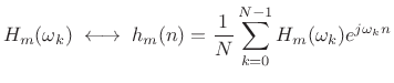
STFT with Modifications
FBS Fixed Modifications
Consider applying a fixed (time-invariant) filter
![]() to
each
to
each
![]() before resynthesizing the signal:
before resynthesizing the signal:
| (10.28) |
where,
 |
(10.29) |
Let's examine the result this has on the signal in the time domain:
![\begin{eqnarray*}
y(m) &=& \frac{1}{N} \sum_{k=0}^{N-1} Y_m(\omega_k) e^{j\omega_k m} \\
&=& \frac{1}{N} \sum_{k=0}^{N-1} X_m(\omega_k)H(\omega_k) e^{j\omega_k m} \\
&=& \frac{1}{N} \sum_{k=0}^{N-1} \left\{ \sum_{n=-\infty}^\infty x(n)w(n-m)e^{-j\omega_kn} \right\} H(\omega_k) e^{j\omega_k m} \\
&=& \frac{1}{N} \sum_{n=-\infty}^\infty x(n)w(n-m) \sum_{k=0}^{N-1} H(\omega_k) e^{j\omega_k(m-n)} \\
&=& \sum_{n=-\infty}^\infty x(n) [ w(n-m) h(m-n)] \\
&=& \sum_{n=-\infty}^\infty x(n) [\tilde{w}(m-n)h(m-n)] \\
&=& (x*[\tilde{w} \cdot h])(m) \\
\end{eqnarray*}](http://www.dsprelated.com/josimages_new/sasp2/img1704.png)
We see that the result is ![]() convolved with a windowed version
of the impulse response
convolved with a windowed version
of the impulse response ![]() . This is in contrast to the OLA technique
where the result gave us a windowed
. This is in contrast to the OLA technique
where the result gave us a windowed ![]() filtered by
filtered by ![]() without the
window having any effect on the filter, provided it obeys the COLA
constraint and sufficient zero padding is used to avoid time aliasing.
without the
window having any effect on the filter, provided it obeys the COLA
constraint and sufficient zero padding is used to avoid time aliasing.
In other words, FBS gives
| (10.30) |
while OLA gives (for
| (10.31) |
- In FBS, the analysis window
 smooths the filter frequency response by time-limiting the corresponding impulse response.
- In OLA, the analysis window can only affect scaling.
For these reasons, FFT implementations of FIR filters normally use the Overlap-Add method.
Time Varying Modifications in FBS
Consider now applying a time varying modification.
| (10.32) |
where
 |
(10.33) |
![\begin{eqnarray*}
y(m) &=& \frac{1}{N} \sum_{k=0}^{N-1} Y_m(\omega_k) e^{j\omega_k m} \\
&=& \frac{1}{N} \sum_{k=0}^{N-1} X_m(\omega_k)H_m(\omega_k) e^{j\omega_k m} \\
&=& \frac{1}{N} \sum_{k=0}^{N-1} \left\{ \sum_{n=-\infty}^\infty x(n)w(n-m)e^{-j\omega_kn} \right\} H_m(\omega_k) e^{j\omega_k m} \\
&=& \frac{1}{N} \sum_{n=-\infty}^\infty x(n)w(n-m) \sum_{k=0}^{N-1} H_m(\omega_k) e^{j\omega_k(m-n)} \\
&=& \sum_{n=-\infty}^\infty x(n) [ w(n-m) h_m(m-n)] \\
&=& \sum_{n=-\infty}^\infty x(n) [\tilde{w}(m-n)h_m(m-n)] \\
&=& (x*[\tilde{w} \cdot h_m])(m) \\
\end{eqnarray*}](http://www.dsprelated.com/josimages_new/sasp2/img1711.png)
Hence, the result is the convolution of ![]() with the windowed
with the windowed ![]() .
.
Points to Note
- We saw that in OLA with time varying modifications and
 (a
``sliding'' DFT), the window served as a lowpass filter on
each individual tap of the FIR filter being implemented.
(a
``sliding'' DFT), the window served as a lowpass filter on
each individual tap of the FIR filter being implemented.
- In the more typical case in which
 is the window length
  divided by a small integer like
  -
- , we may think of the window as
specifying a type of cross-fade from the LTI filter for one
frame to the LTI filter for the next frame.
, we may think of the window as
specifying a type of cross-fade from the LTI filter for one
frame to the LTI filter for the next frame.
- Using a Bartlett (triangular) window with
 % overlap,
(
% overlap,
( ), the sequence of FIR filters used is obtained simply by
linearly interpolating the LTI filter for one frame to the LTI
filter for the next.
), the sequence of FIR filters used is obtained simply by
linearly interpolating the LTI filter for one frame to the LTI
filter for the next.
- In FBS, there is no limitation on how fast the filter
 may vary with time,
but its length is limited to that of the window
.
may vary with time,
but its length is limited to that of the window
.
- In OLA, there is no limit on length (just add more zero-padding), but
the filter taps are band-limited to the spectral width of the window.
- FBS filters are time-limited by
, while OLA
filters are band-limited by
(another dual relation).
- Recall for comparison that each frame in the OLA method is filtered
according to
![$\displaystyle Y_m = X_m \cdot H_m = [X*W_m] \cdot H_m \;\longleftrightarrow\; \underbrace{[x \cdot w_m]}_{x_m} * h_m$](http://www.dsprelated.com/josimages_new/sasp2/img1713.png)
(10.34)
where denotes
 .
.
- Time-varying FBS filters are instantly in ``steady state''
- FBS filters must be changed very slowly to avoid clicks and pops (discontinuity distortion is likely when the filter changes)
STFT Summary and Conclusions
The Short-Time Fourier Transform (STFT) may be viewed either as an OverLap-Add (OLA) processor, or as a Filter-Bank Sum (FBS). We derived two conditions for perfect reconstruction which are Fourier duals of each other:
- For OLA, the window must overlap-add to a constant in the time
domain. By the Poisson summation formula, this is equivalent
to having window transform nulls at all nonzero multiples of
the frame rate
 .
.
- For FBS, the window transform must overlap-add to a
constant in the frequency domain, and this is equivalent to
having window nulls in the time domain at all nonzero multiples
of the transform size
 .
.
In general, STFT filter banks are oversampled except when using
the rectangular window of length ![]() and a hop size
and a hop size ![]() . Critical
sampling is desirable for compression systems, but this can be
problematic when spectral modifications are contemplated
(adjacent-channel aliasing no longer canceled).
. Critical
sampling is desirable for compression systems, but this can be
problematic when spectral modifications are contemplated
(adjacent-channel aliasing no longer canceled).
STFT filter banks are uniform filter banks, as opposed ``constant Q''. In some audio applications, it is preferable to use non-uniform filter banks which approximate the auditory filter bank. Approximate constant-Q filter banks are easily synthesized from STFT filter banks by summing adjacent frequency channels, as detailed in §10.7 below. Additional pointers can be found in Appendix E. We will look at a particular octave filter bank when we talk about wavelet filter banks (§11.9).
Next Section:
Applications of the STFT
Previous Section:
Overlap-Add (OLA) STFT Processing


