DSPRelated.com
Free Books

Hilbert Transform

The Hilbert transform $ y(t)$ of a real, continuous-time signal $ x(t)$ may be expressed as the convolution of $ x$ with the Hilbert transform kernel:

$\displaystyle h(t) \isdefs \frac{1}{\pi t},\qquad t\in(-\infty,\infty) \protect$ (5.17)

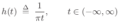
That is, the Hilbert transform of $ x$ is given by

$\displaystyle y = h \ast x. % \qquad \hbox{(Hilbert transform of $x$)}.
$ (5.18)

Thus, the Hilbert transform is a non-causal linear time-invariant filter.

The complex analytic signal $ x_a(t)$ corresponding to the real signal $ x(t)$ is then given by

$\displaystyle x_a(t)$ $\displaystyle \isdef$ $\displaystyle x(t) + j y(t)$  
$\displaystyle %\qquad \hbox{(Analytic signal corresponding to $x$)}\\ [10pt]
$ $\displaystyle =$ $\displaystyle \frac{1}{\pi}\displaystyle\int_0^{\infty} X(\omega)e^{j\omega t}\, d\omega$ (5.19)

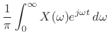
To show this last equality (note the lower limit of 0 instead of the usual $ -\infty$ ), it is easiest to apply (4.16) in the frequency domain:

$\displaystyle X_a(\omega)$ $\displaystyle \isdef$ $\displaystyle X(\omega) + j Y(\omega)$  
  $\displaystyle \isdef$ $\displaystyle (X_++X_-) + j (-j X_+ + j X_-)$ (5.20)
  $\displaystyle =$ $\displaystyle 2X_+(\omega)$ (5.21)

Thus, the negative-frequency components of $ X$ are canceled, while the positive-frequency components are doubled. This occurs because, as discussed above, the Hilbert transform is an allpass filter that provides a $ 90$ degree phase shift at all negative frequencies, and a $ -90$ degree phase shift at all positive frequencies, as indicated in (4.16). The use of the Hilbert transform to create an analytic signal from a real signal is one of its main applications. However, as the preceding sections make clear, a Hilbert transform in practice is far from ideal because it must be made finite-duration in some way.


Next Section:
Matlab, Continued
Previous Section:
Comparison to the Optimal Chebyshev FIR Bandpass Filter