


A History of Spectral Audio Signal Processing
This appendix surveys some of the highlights of developments in spectral audio signal processing, beginning with Daniel Bernoulli's original understanding of acoustic vibration as a superposition of sinusoidally vibrating modes and progressing through more recent history in spectral modeling of audio signals. A complete history of audio spectral models would be a very large undertaking. Instead, this appendix offers a sequence of what the author considers to be interesting and important topics in more or less chronological order.
Daniel Bernoulli's Modal Decomposition
The history of spectral modeling of sound arguably begins with Daniel Bernoulli, who first believed (in the 1733-1742 time frame) that any acoustic vibration could be expressed as a superposition of ``simple modes'' (sinusoidal vibrations) [52].G.1Bernoulli was able to show this precisely for the case of identical masses interconnected by springs to form a discrete approximation to an ideal string. Leonard Euler first wrote down (1749) a mathematical expression of Bernoulli's insight for a special case of the continuous vibrating string:
 |
(G.1) |
Euler's paper was primarily in response to d'Alembert's landmark derivation (1747) of the traveling-wave picture of vibrating strings [266], which showed that vibrating string motion could assume essentially any twice-differentiable shape. Euler did not consider Bernoulli's sinusoidal superposition to be mathematically complete because clearly a trigonometric sum could not represent an arbitrary string shape.G.2D'Alembert did not believe that a superposition of sinusoids could be ``physical'' in part because he imagined what we would now call ``intermodulation distortion'' due to a high-frequency component ``riding on'' a lower-frequency component (as happens nowadays in loudspeakers).G.3 Arguments over the generality of the sinusoidal expansion of string vibration persisted for decades, embroiling also Lagrange, and were not fully settled until Fourier theory itself was wrestled into submission by the development of distribution theory, measure theory, and the notion of convergence ``almost everywhere.''
Note that organ builders had already for centuries built machines for performing a kind of ``additive synthesis'' by gating various ranks of pipes using ``stops'' as in pipe organs found today. However, the waveforms mixed together were not sinusoids, and were not regarded as mixtures of sinusoids. Theories of sound at that time, based on the ideas of Galileo, Mersenne, and Sauveur, et al. [52], were based on time-domain pulse-train analysis. That is, an elementary tone at a fixed pitch (and fundamental frequency) was a periodic pulse train, with the pulse-shape being non-critical. Musical consonance was associated with pulse-train coincidence--not frequency-domain separation. Bernoulli clearly suspected the spectrum analysis function integral to hearing as well as color perception [52, p. 359], but the concept of the ear as a spectrum analyzer is generally attributed to Helmholtz (1863) [293].
The Telharmonium
The Telharmonium was a machine for generating a kind of ``additive synthesis'' of musical sound for distribution over telephone lines. It is described in U.S. patent 580,035 by Thaddeus Cahill (1898), entitled ``Art of and Apparatus for Generating and Distributing Music Electrically''
![\includegraphics[width=\twidth]{eps/th-rheo1}](http://www.dsprelated.com/josimages_new/sasp2/img2976.png)
![\includegraphics[width=0.7\twidth]{eps/th-rheo2}](http://www.dsprelated.com/josimages_new/sasp2/img2977.png)
Sound was generated electromechanically in the Telharmonium by so-called rheotomes, depicted in Figures G.1 and G.2 from the patent. A rheotome was a spinning metal shaft with cut-outs that caused a periodic electrical signal to be picked up by capacitive coupling. The rheotome is a clear forerunner of the Hammond organ tone wheels, shown in Fig.G.3.
Because rheotomes did not generate sinusoidal components, the Telharmonium is better considered an electromechanical descendant of the pipe organ than as an ``additive synthesis'' device in the modern sense (i.e., inspired by Bernoulli's modal decomposition insight and Fourier's famous theorem). However, the Hammond organ was conceptually an additive synthesis device (having drawbars on individual overtones), and it was clearly influenced by the Telharmonium.
Early Additive Synthesis in Film Making
In the 1930s, Russian ``futurists'' used ``syntones''' to synthesize film soundtracks by means of a sum of sinusoidal components [257]. (Fourier transforms for analyzing periodic sounds had to be carried out by hand.) Artificial synthesis of film soundtracks employed professional animators to ``draw'' sounds directly to produce photographic masks.G.4
The Hammond Organ
The Hammond organ was introduced in US Patent 1,956,350. A difference between the Hammond organ and Telharmonium is that Telharmonium tones were something like ``bandlimited square wave'' tones (see Fig.G.1), while the Hammond organ tone wheels were carefully machined to provide nearly sinusoidal components. Thus, the Hammond organ truly classifies as an ``additive synthesis device'' (§G.8). It has survived essentially intact to the present day, and has been extensively simulated electronically (e.g., in Korg synthesizers).
![\includegraphics[width=0.7\twidth]{eps/tonewheels}](http://www.dsprelated.com/josimages_new/sasp2/img2978.png)
Dudley's Channel Vocoder
The first major effort to encode speech electronically was Homer Dudley's channel vocoder (``voice coder'') [68] developed starting in October of 1928 at AT&T Bell Laboratories [245]. An overall schematic of the channel vocoder is shown in Fig.G.4.
![\begin{psfrags}
% latex2html id marker 41913\psfrag{x} []{ \LARGE$ x(t)$\ }\psfrag{X0} []{ \LARGE$ x_0(t) $\ }\psfrag{X1} []{ \LARGE$ x_1(t)$\ }\psfrag{XNM1} []{ \LARGE$ x_{N-1}(t)$\ }\psfrag{xhat} []{ \LARGE$ \hat{x}(t)$\ }\psfrag{Xhat0} []{ \LARGE$ \hat{x}_0(t) $\ }\psfrag{Xhat1} []{ \LARGE$ \hat{x}_1(t)$\ }\psfrag{XhatNM1} []{ \LARGE$ \hat{x}_{N-1}(t)$\ }\begin{figure}[htbp]
\includegraphics[width=\twidth]{eps/vocoder}
\caption{Channel or phase vocoder block diagram.}
\end{figure}
\end{psfrags}](http://www.dsprelated.com/josimages_new/sasp2/img2979.png)
On analysis, the outputs of ten analog bandpass filters (spanning
250-3000 Hz)G.5were rectified and lowpass-filtered to obtain amplitude envelopes for
each band. In parallel, the fundamental frequency ![]() was measured,
and a voiced/unvoiced decision was made (unvoiced segments were
indicated by
was measured,
and a voiced/unvoiced decision was made (unvoiced segments were
indicated by ![]() . On synthesis, a ``buzz source'' (relaxation
oscillator) at pitch
. On synthesis, a ``buzz source'' (relaxation
oscillator) at pitch ![]() (for voiced speech) or a ``hiss source''
(for unvoiced speech) was used to drive a set of ten matching bandpass
filters, whose outputs were summed to produce the reconstructed voice.
While the voice quality had a quite noticeable ``unpleasant electrical
accent'' [245],
the bandwidth required to transmit
(for voiced speech) or a ``hiss source''
(for unvoiced speech) was used to drive a set of ten matching bandpass
filters, whose outputs were summed to produce the reconstructed voice.
While the voice quality had a quite noticeable ``unpleasant electrical
accent'' [245],
the bandwidth required to transmit
![]() and the bandpass-filter gain envelopes was much less than
that required to transmit the original speech signal.
and the bandpass-filter gain envelopes was much less than
that required to transmit the original speech signal.
The vocoder synthesis model can be considered a
source-filter model for speech which uses a
nonparametric spectral model of the vocal tract given by the
output of a fixed bandpass-filter-bank over time. Related efforts
included the formant vocoder [190]--a
type of parametric spectral model--which encoded ![]() and the
amplitude and center-frequency of the first three spectral
formants. See [168, pp. 2452-3] for an overview and
references.
and the
amplitude and center-frequency of the first three spectral
formants. See [168, pp. 2452-3] for an overview and
references.
The original vocoder used a ``buzz source'' (implemented using ``relaxation oscillator'') driving the filter bank during voiced speech, and a ``hiss source'' (implemented using the noise from a resistor) driving the filter bank during unvoiced speech. In later speech modeling by linear-prediction [162], the buzz source evolved to the more mathematically pure impulse train, and the hiss source became white noise.
The vocoder used an analog bandpass filter bank, and only the amplitude envelope was retained for each bandpass channel. When the vocoder was later reimplemented using the discrete Fourier transform on a digital computer (§G.7 below), it became simple to record both the instantaneous amplitude and phase for each channel. As a result, the name was updated to phase vocoder. Section G.7 summarizes the history of the phase vocoder, and §G.10 describes an example implementation using the STFT.
Speech Synthesis Examples
The original goal of the vocoder was speech synthesis from a sparse, parametric model. A large collection of sound examples spanning the history of speech synthesis can be heard on the CD-ROM accompanying a JASA-87 review article by Dennis Klatt [129].
Voder
The Voder was a manually driven speech synthesizer developed by Homer Dudley at Bell Telephone Laboratories. Details are described in US Patent 2,121,142 (filed 1937). The Voder was demonstrated at the 1939 World's Fair.
The voder was manually operated by trained technicians.G.6Pitch was controlled by a foot pedal, and ten fingers controlled the bandpass gains. Buzz/hiss selection was by means of a wrist bar. Three additional keys controlled transient excitation of selected filters to achieve stop-consonant sounds [75]. ``Performing speech'' on the Voder required on the order of a year's training before intelligible speech could reliably be produced. The Voder was a versatile performing instrument having intriguing possibilities well beyond voice synthesis.
Phase Vocoder
In the 1960s, the phase vocoder was introduced by Flanagan and Golden
based on interpreting the classical vocoder (§G.5) filter
bank as a sliding short-time Fourier transform
[76,243]. The digital computer made
it possible for the phase vocoder to easily support phase modulation
of the synthesis oscillators as well as implementing their amplitude
envelopes. Thus, in addition to computing the instantaneous amplitude
at the output of each (complex) bandpass filter, the instantaneous
phase was also computed. (Phase could be converted to frequency by
taking a time derivative.) Complex bandpass filters were implemented
by multiplying the incoming signal by
![]() , where
, where
![]() is the
is the ![]() th channel radian center-frequency, and
lowpass-filtering using a sixth-order Bessel filter.
th channel radian center-frequency, and
lowpass-filtering using a sixth-order Bessel filter.
The phase vocoder also relaxed the requirement of pitch-following (needed in the vocoder), because the phase modulation computed by the analysis stage automatically fine-tuned each sinusoidal component within its filter-bank channel. The main remaining requirement was that only one sinusoidal component be present in any given channel of the filter bank; otherwise, the instantaneous amplitude and frequency computations would be based on ``beating'' waveforms instead of single quasi-sinusoids which produce smooth amplitude and frequency envelopes necessary for good data compression.
Unlike the hardware implementations of the channel vocoder, the phase vocoder is typically implemented in software on top of a Short-Time Fourier Transform (STFT), and originally reconstructed the signal from its amplitude spectrum and ``phase derivative'' (instantaneous frequency) spectrum [76]. Time scale modification (§10.5) and frequency shifting were early applications of the phase vocoder [76].
The phase vocoder can also be considered an early subband coder [284]. Since the mid-1970s, subband coders have typically been implemented using the STFT [76,212,9]. In the field of perceptual audio coding, additional compression has been obtained using undersampled filter banks that provide aliasing cancellation [287], the first example being the Princen-Bradley filter bank [214].
The phase vocoder was also adopted as the analysis framework of choice for additive synthesis (later called sinusoidal modeling) in computer music [186]. (See §G.8, for more about additive synthesis.)
Today, the term ``vocoder'' has become somewhat synonymous in the audio research world with ``modified short-time Fourier transform'' [212,62]. In the commercial musical instrument world, it connotes a keyboard instrument with a microphone that performs cross-synthesis (§10.2).
FFT Implementation of the Phase Vocoder
In the 1970s, the phase vocoder was reimplemented using the FFT for increased computational efficiency [212]. The FFT window (analysis lowpass filter) was also improved to yield exact reconstruction of the original signal when synthesizing without modifications. Shortly thereafter, the FFT-based phase-vocoder became the basis for additive synthesis in computer music [187,62]. A generic diagram of phase-vocoder (or vocoder) processing is given in Fig.G.4. Since then, numerous variations and improvements of the phase vocoder have appeared, e.g., [99,215,140,138,143,142,139]. A summary of vocoder research from the 1930s to the 60s appears in a review article by Manfred Schroeder [245]. The phase vocoder and its descendants (STFT modification/resynthesis, sinusoidal modeling) have been used for many audio applications, such as speech coding and transmission, data compression, noise reduction, reverberation suppression, cross-synthesis (§10.2), time scale modification (§10.5), frequency shifting, and much more.
Additive Synthesis
Additive synthesis (now more often called ``sinusoidal modeling'') was one of the first computer-music synthesis methods, and it has been a mainstay ever since. In fact, it is extensively described in the first article of the first issue of the Computer Music Journal [186]. Some of the first high-quality synthetic musical instrument tones using additive synthesis were developed in the 1960s by Jean-Claude Risset at AT&T Bell Telephone Laboratories [233,232].
Additive synthesis was historically implemented using a sum of sinusoidal oscillators modulated by amplitude and frequency envelopes over time [186], and later using an inverse FFT [35,239] when the number of sinusoids is large.
Figure G.5 shows an example from John Grey's 1975 Ph.D. thesis (Psychology) illustrating the nature of partial amplitude envelopes computed for purposes of later resynthesis.
![\includegraphics[width=0.8\twidth]{eps/grey-anal}](http://www.dsprelated.com/josimages_new/sasp2/img2983.png) |
Inverse FFT Synthesis
When the number of partial overtones is large, an explicit sinusoidal oscillator bank requires a significant amount of computation, and it becomes more efficient to use the inverse FFT to synthesize large ensembles of sinusoids [35,239,143,142,139]. This method gives the added advantage of allowing non-sinusoidal components such as filtered noise to be added in the frequency domain [246,249].
Inverse-FFT (IFFT) synthesis was apparently introduced by Hal Chamberlin in his classic 1980 book ``Musical Applications of Microprocessors'' [35]. His early method consisted of simply setting individual FFT bins to the desired amplitude and phase, so that an inverse FFT would efficiently synthesize a sum of fixed-amplitude, fixed-frequency sinusoids in the time domain.
This idea was extended by Rodet and Depalle [239] to
include shaped amplitudes in the time domain. Instead of
writing isolated FFT bins, they wrote entire main lobes into
the buffer, where the main lobes corresponded to the desired window
shape in the time domain.G.7 (Side
lobes of the window transform were neglected.) They chose the
triangular window (
![]() main-lobe shape), thereby implementing a
linear cross-fade from one frame to the next in the time domain.
main-lobe shape), thereby implementing a
linear cross-fade from one frame to the next in the time domain.
A remaining drawback of IFFT synthesis was that inverse FFTs generate sinusoids at fixed frequencies, so that a rapid glissando may become ``stair-cased'' in the resynthesis, stepping once in frequency per output frame.
An extension of IFFT synthesis to support linear frequency sweeps was devised by Goodwin and Kogon [93]. The basic idea was to tabulate window main-lobes for a variety of sweep rates. (The phase variation across the main lobe determines the frequency variation over time, and the width of the main lobe determines its extent.) In this way, frequencies could be swept within an FFT frame instead of having to be constant with a cross-fade from one static frame to the next.
Chirplet Synthesis
Independently of Goodwin and Kogon, Marques and Almeida introduced chirplet modeling of speech in 1989 [164]. This technique is based on the interesting mathematical fact that the Fourier transform of a Gaussian-windowed chirp remains a Gaussian pulse in the frequency domain (§10.6). Instead of measuring only amplitude and phase at each a spectral peak, the parameters of a complex Gaussian are fit to each peak. The (complex) parameters of each Gaussian peak in the spectral model determine a Gaussian amplitude-envelope and a linear chirp rate in the time domain. Thus, both cross-fading and frequency sweeping are handled automatically by the spectral model. A specific method for carrying this out is described in §10.6. More recent references on chirplet modeling include [197,90,91,89].
Nonparametric Spectral Peak Modeling
Beginning in 1999, Laroche and Dolson extended IFFT synthesis (§G.8.1) further by using raw spectral-peak regions from STFT analysis data [143,142,139]. By preserving the raw spectral peak (instead of modeling it mathematically as a window transform or complex Gaussian function), the original amplitude envelope and frequency variation are preserved for the signal component corresponding to the analyzed peak in the spectrum. To implement frequency-shifting, for example, the raw peaks (defined as ``regions of influence'' around a peak-magnitude bin) are shifted accordingly, preserving the original amplitude and phase of the FFT bins within each peak region.
Efficient Specialized Methods
We have already mentioned inverse-FFT synthesis as a means of greatly decreasing the cost of additive synthesis relative to a full-blown bank of sinusoidal oscillators. This section summarizes a number of more specialized methods which reduce the computational cost of additive synthesis and are widely used.
Wavetable Synthesis
For periodic sounds, the sinusoidal components are all harmonics of some fundamental frequency. If in addition they can be constrained to vary together in amplitude over time, then they can be implemented using a single wavetable containing one period of the sound. Amplitude shaping is handled by multiplying the output of the wavetable look-up by an amplitude-envelope generated separately [186,167]. Using interpolation (typically linear, but sometimes better), the table may be played back at any fundamental frequency, and its output is then multiplied by the amplitude envelope shared by all harmonics. (The harmonics may still have arbitrary relative levels.) This form of ``wavetable synthesis'' was commonly used in the early days of computer music. This method is still commonly used for synthesizing harmonic spectra.G.8
Note that sometimes the term ``wavetable synthesis'' is used to refer to what was originally called sampling synthesis: playback of sampled tones from memory, with looping of the steady-state portion to create an arbitrarily long sustain [165,27,107,193]. This book adheres to the original terminology. For sampling synthesis, spectral phase-modifications (Chapter 8) can be used to provide perfectly seamless loops [165].
Group-Additive Synthesis
The basic idea of group-additive synthesis [130,69] is to employ a set of wavetables, each modeling a harmonic subset of the tonal components making up the overall spectrum of the synthesized tone. Since each wavetable oscillator is independent, inharmonic sounds can be synthesized to some degree of approximation, and the amplitude envelopes are not completely locked together. It is important to be aware that human audio perception cannot tell the difference between harmonic and inharmonic partials at high frequencies (where ``high'' depends on the fundamental frequency and timbre to some extent). Thus, group-additive synthesis provides a set of intermediate points between wavetable synthesis and all-out additive synthesis.
Further Reading, Additive Synthesis
For more about the history of additive synthesis, see the chapter on ``Sampling and Additive Synthesis'' in [235]. For ``hands-on'' introductions to additive synthesis (with examples in software), see [216] (pd), [60] (Csound [19]), or [183] (cmusic). A discussion of the phase vocoder in conjunction with additive synthesis begins in §G.10.
Frequency Modulation (FM) Synthesis
The first commercial digital sound synthesis method was Frequency Modulation (FM) synthesis [38,41,39], invented by John Chowning, the founding director of CCRMA. FM synthesis was discovered and initially developed in the 1970s [38]. The technology was commercialized by Yamaha Corporation, resulting in the DX-7 (1983), the first commercial digital music synthesizer, and the OPL chipset, initially in the SoundBlaster PC sound card, and later a standard chipset required for ``SoundBlaster compatibility'' in computer multimedia support. The original pioneer patent expired in 1996, but additional patents were filed later. It is said that this technology lives on in cell-phone ring-tone synthesis.
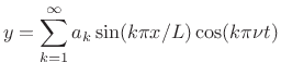
As discussed more fully in [264, p. 44], the formula for elementary FM synthesis is given by
where An example computer-music-style diagram is shown in Fig.G.6. Since the instantaneous frequency of a sinusoid is simply the time-derivative of its instantaneous phase, FM can also be regarded as phase modulation (PM). It is highly remarkable that such a simple algorithm can generate such a rich variety of musically useful sounds. This is probably best understood by thinking of FM as a spectral modeling technique, as will be illustrated further below.

FM Harmonic Amplitudes (Bessel Functions)
FM bandwidth expands as the modulation-amplitude ![]() is increased
in (G.2) above. The
is increased
in (G.2) above. The ![]() th harmonic amplitude is proportional to
the
th harmonic amplitude is proportional to
the ![]() th-order Bessel function of the first kind
th-order Bessel function of the first kind ![]() , evaluated at
the
FM modulation index
, evaluated at
the
FM modulation index
![]() . Figure G.7 illustrates
the behavior of
. Figure G.7 illustrates
the behavior of
![]() : As
: As ![]() is increased, more power
appears in the sidebands, at the expense of the fundamental. Thus,
increasing the FM index brightens the tone.
is increased, more power
appears in the sidebands, at the expense of the fundamental. Thus,
increasing the FM index brightens the tone.
![\includegraphics[width=\twidth]{eps/bessel}](http://www.dsprelated.com/josimages_new/sasp2/img2992.png) |
FM Brass
Jean-Claude Risset observed (1964-1969), based on spectrum analysis of brass tones [233], that the bandwidth of a brass instrument tone was roughly proportional to its overall amplitude. In other words, the spectrum brightened with amplitude. This observation inspired John Chowning's FM brass synthesis technique (starting in 1970[40]). For FM brass, the FM index is made proportional to carrier amplitude, thus yielding a dynamic brightness variation with amplitude that sounds consistently ``brassy''. A simple example of an FM brass instrument is shown in Fig.G.6 above. Note how the FM index is proportional to the amplitude envelope (carrier amplitude).
FM Voice
FM voice synthesis [39] can be viewed as compressed modeling of spectral formants. Figure G.8 shows the general idea. This kind of spectral approximation was used by John Chowning and others at CCRMA in the 1980s and beyond to develop convincing voices using FM. Another nice example was the FM piano developed by John Chowning and David Bristow [41].
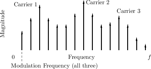
A basic
FM operator,
consisting of two sinusoidal oscillators
(a ``modulator'' and a ``carrier'' oscillator, as written
in Eq.![]() (G.2)), can synthesize a useful approximation to
a formant group in a harmonic line spectrum. In this
technique, the carrier frequency is set near the formant center
frequency, rounded to the nearest harmonic frequency, and the
modulating frequency is set to the desired pitch (e.g., of a sung
voice [39]). The modulation index is set to give the
desired bandwidth for the formant group. For the singing
voice, three or more formant groups yields a
sung vowel sound. Thus, a sung vowel can be synthesized using
only six sinusoidal oscillators using FM. In straight additive
synthesis, a bound on the number of oscillators needed is given by the
upper band-limit divided by the fundamental frequency, which could be,
for a strongly projecting deep male voice, on the order of
(G.2)), can synthesize a useful approximation to
a formant group in a harmonic line spectrum. In this
technique, the carrier frequency is set near the formant center
frequency, rounded to the nearest harmonic frequency, and the
modulating frequency is set to the desired pitch (e.g., of a sung
voice [39]). The modulation index is set to give the
desired bandwidth for the formant group. For the singing
voice, three or more formant groups yields a
sung vowel sound. Thus, a sung vowel can be synthesized using
only six sinusoidal oscillators using FM. In straight additive
synthesis, a bound on the number of oscillators needed is given by the
upper band-limit divided by the fundamental frequency, which could be,
for a strongly projecting deep male voice, on the order of ![]() kHz
divided by 100 Hz, or 200 oscillators.
kHz
divided by 100 Hz, or 200 oscillators.
Today, FM synthesis is still a powerful spectral modeling technique in which ``formant harmonic groups'' are approximated by the spectrum of an elementary FM oscillator pair. This remains a valuable tool in environments where memory access is limited, such as in VLSI chips used in hand-held devices, as it requires less memory than wavetable synthesis (§G.8.4).
In the context of audio coding, FM synthesis can be considered a ``lossy compression method'' for additive synthesis.
Further Reading about FM Synthesis
For further reading about FM synthesis, see the original Chowning paper [38], paper anthologies including FM [236,234], or just about any computer-music text [235,183,60,216].
Phase Vocoder Sinusoidal Modeling
As mentioned in §G.7, the phase vocoder had become a standard analysis tool for additive synthesis (§G.8) by the late 1970s [186,187]. This section summarizes that usage.
In analysis for additive synthesis, we convert a time-domain signal
![]() into a collection of amplitude envelopes
into a collection of amplitude envelopes ![]() and frequency envelopes
and frequency envelopes
![]() (or phase modulation envelopes
(or phase modulation envelopes
![]() ), as graphed in Fig.G.12.
It is usually desired that these envelopes be slowly varying
relative to the original signal. This leads to the assumption that we
have at most one sinusoid in each filter-bank channel. (By
``sinusoid'' we mean, of course, ``quasi sinusoid,'' since its
amplitude and phase may be slowly time-varying.) The channel-filter
frequency response is given by the FFT of the analysis window used
(Chapter 9).
), as graphed in Fig.G.12.
It is usually desired that these envelopes be slowly varying
relative to the original signal. This leads to the assumption that we
have at most one sinusoid in each filter-bank channel. (By
``sinusoid'' we mean, of course, ``quasi sinusoid,'' since its
amplitude and phase may be slowly time-varying.) The channel-filter
frequency response is given by the FFT of the analysis window used
(Chapter 9).
The signal in the ![]() subband (filter-bank channel) can be
written
subband (filter-bank channel) can be
written
In this expression,
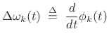
Typically, the instantaneous phase modulation ![]() is
differentiated to obtain instantaneous frequency deviation:
is
differentiated to obtain instantaneous frequency deviation:
 |
(G.4) |
The analysis and synthesis signal models are summarized in Fig.G.9.
![\includegraphics[width=\twidth]{eps/pvchan}](http://www.dsprelated.com/josimages_new/sasp2/img3000.png)
Computing Vocoder Parameters
To compute the amplitude ![]() at the output of the
at the output of the ![]() th subband,
we can apply an envelope follower. Classically, such as in the
original vocoder, this can be done by full-wave rectification and
subsequent low pass filtering, as shown in Fig.G.10. This
produces an approximation of the average power in each subband.
th subband,
we can apply an envelope follower. Classically, such as in the
original vocoder, this can be done by full-wave rectification and
subsequent low pass filtering, as shown in Fig.G.10. This
produces an approximation of the average power in each subband.
![\begin{psfrags}
% latex2html id marker 42527\psfrag{x} []{ \LARGE$ x_k(t)$\ }\psfrag{xkt} []{ \LARGE$ \tilde{x}_k(t)$\ }\psfrag{xk} []{ \LARGE$ x_k(t)$\ }\psfrag{output} []{ \LARGE$ y_k=h*\tilde{x}_k $\ }\begin{figure}[htbp]
\includegraphics[width=\textwidth ]{eps/envelope}
\caption{Classic method for amplitude envelope
extraction in continuous-time analog circuits.}
\end{figure}
\end{psfrags}](http://www.dsprelated.com/josimages_new/sasp2/img3001.png)
In digital signal processing, we can do much better than the classical amplitude-envelope follower: We can measure instead the instantaneous amplitude of the (assumed quasi sinusoidal) signal in each filter band using so-called analytic signal processing (introduced in §4.6). For this, we generalize (G.3) to the real-part of the corresponding analytic signal:
In general, when both amplitude and phase are needed, we must compute two real signals for each vocoder channel:
![$\displaystyle \tan^{-1} \left[ \frac{\mbox{im\ensuremath{\left\{x_k^a(t)\right\}}}}
{\mbox{re\ensuremath{\left\{x_k^a(t)\right\}}}} \right] - \omega_kt
\protect$](http://www.dsprelated.com/josimages_new/sasp2/img3011.png)
We call
In order to determine these signals, we need to compute the analytic
signal ![]() from its real part
from its real part ![]() . Ideally, the imaginary
part of the analytic signal is obtained from its real part using
the Hilbert transform (§4.6), as shown
in Fig.G.11.
. Ideally, the imaginary
part of the analytic signal is obtained from its real part using
the Hilbert transform (§4.6), as shown
in Fig.G.11.
![\begin{psfrags}
% latex2html id marker 42563\psfrag{x} []{ \LARGE$ x_k(t)$\ }\psfrag{Rex} []{ \LARGE$ \mbox{re\ensuremath{\left\{x_k^a(t)\right\}}}$\ }\psfrag{Imx} []{ \LARGE$ \mbox{im\ensuremath{\left\{x_k^a(t)\right\}}}$\ }\begin{figure}[htbp]
\includegraphics[width=0.8\twidth]{eps/hilbert}
\caption{Creating an analytic signal
from its real part using the Hilbert transform
(\textit{cf.}{} \sref {hilbert}).}
\end{figure}
\end{psfrags}](http://www.dsprelated.com/josimages_new/sasp2/img3015.png)
Using the Hilbert-transform filter, we obtain the analytic signal in ``rectangular'' (Cartesian) form:
| (G.7) |
To obtain the instantaneous amplitude and phase, we simply convert each complex value of
| (G.8) |
as given by (G.6).
Frequency Envelopes
It is convenient in practice to work with instantaneous frequency deviation instead of phase:
|
(G.9) |
Since the
Note that ![]() is a narrow-band signal centered about the channel
frequency
is a narrow-band signal centered about the channel
frequency ![]() . As detailed in Chapter 9, it is typical
to heterodyne the channel signals to ``base band'' by shifting
the input spectrum by
. As detailed in Chapter 9, it is typical
to heterodyne the channel signals to ``base band'' by shifting
the input spectrum by ![]() so that the channel bandwidth is
centered about frequency zero (dc). This may be expressed by
modulating the analytic signal by
so that the channel bandwidth is
centered about frequency zero (dc). This may be expressed by
modulating the analytic signal by
![]() to get
to get
 |
(G.10) |
The `b' superscript here stands for ``baseband,'' i.e., the channel-filter frequency-response is centered about dc. Working at baseband, we may compute the frequency deviation as simply the time-derivative of the instantaneous phase of the analytic signal:
 |
(G.11) |
where
 |
(G.12) |
denotes the time derivative of
 |
(G.13) |
For discrete time, we replace
Initially, the sliding FFT was used (hop size
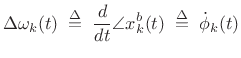
Using (G.6) and (G.14) to compute the instantaneous amplitude and frequency for each subband, we obtain data such as shown qualitatively in Fig.G.12. A matlab algorithm for phase unwrapping is given in §F.4.1.
![\begin{psfrags}
% latex2html id marker 42622\psfrag{ak} []{ \LARGE$ a_k(t)$\ }\psfrag{wkt} []{ \LARGE$ \Delta\omega_k(t)=\dot{\phi_k}(t) $\ }\psfrag{wk} []{ \LARGE$ 0 $\ }\psfrag{t} []{ \LARGE$ t$\ }\begin{figure}[htbp]
\includegraphics[width=3.5in]{eps/traj}
\caption{Example amplitude envelope (top)
and frequency envelope (bottom).}
\end{figure}
\end{psfrags}](http://www.dsprelated.com/josimages_new/sasp2/img3033.png)
Envelope Compression
Once we have our data in the form of amplitude and frequency envelopes
for each filter-bank channel, we can compress them by a large factor.
If there are ![]() channels, we nominally expect to be able to
downsample by a factor of
channels, we nominally expect to be able to
downsample by a factor of ![]() , as discussed initially in Chapter 9
and more extensively in Chapter 11.
, as discussed initially in Chapter 9
and more extensively in Chapter 11.
In early computer music [97,186], amplitude and frequency envelopes were ``downsampled'' by means of piecewise linear approximation. That is, a set of breakpoints were defined in time between which linear segments were used. These breakpoints correspond to ``knot points'' in the context of polynomial spline interpolation [286]. Piecewise linear approximation yielded large compression ratios for relatively steady tonal signals.G.10For example, compression ratios of 100:1 were not uncommon for isolated ``toots'' on tonal orchestral instruments [97].
A more straightforward method is to simply downsample each envelope by
some factor. Since each subband is bandlimited to the channel
bandwidth, we expect a downsampling factor on the order of the number
of channels in the filter bank. Using a hop size ![]() in the STFT
results in downsampling by the factor
in the STFT
results in downsampling by the factor ![]() (as discussed
in §9.8). If
(as discussed
in §9.8). If ![]() channels are downsampled by
channels are downsampled by ![]() , then the
total number of samples coming out of the filter bank equals the
number of samples going into the filter bank. This may be called
critical downsampling, which is invariably used in filter banks
for audio compression, as discussed further in Chapter 11. A benefit
of converting a signal to critically sampled filter-bank form is that
bits can be allocated based on the amount of energy in each subband
relative to the psychoacoustic masking threshold in that band.
Bit-allocation is typically different for tonal and noise signals in a
band [113,25,16].
, then the
total number of samples coming out of the filter bank equals the
number of samples going into the filter bank. This may be called
critical downsampling, which is invariably used in filter banks
for audio compression, as discussed further in Chapter 11. A benefit
of converting a signal to critically sampled filter-bank form is that
bits can be allocated based on the amount of energy in each subband
relative to the psychoacoustic masking threshold in that band.
Bit-allocation is typically different for tonal and noise signals in a
band [113,25,16].
Vocoder-Based Additive-Synthesis Limitations
Using the phase-vocoder to compute amplitude and frequency envelopes for additive synthesis works best for quasi-periodic signals. For inharmonic signals, the vocoder analysis method can be unwieldy: The restriction of one sinusoid per subband leads to many ``empty'' bands (since radix-2 FFT filter banks are always uniformly spaced). As a result, we have to compute many more filter bands than are actually needed, and the empty bands need to be ``pruned'' in some way (e.g., based on an energy detector within each band). The unwieldiness of a uniform filter bank for tracking inharmonic partial overtones through time led to the development of sinusoidal modeling based on the STFT, as described in §G.11.2 below.
Another limitation of the phase-vocoder analysis was that it did not capture the attack transient very well in the amplitude and frequency envelopes computed. This is because an attack transient typically only partially filled an STFT analysis window. Moreover, filter-bank amplitude and frequency envelopes provide an inefficient model for signals that are noise-like, such as a flute with a breathy attack. These limitations are addressed by sinusoidal modeling, sines+noise modeling, and sines+noise+transients modeling, as discussed starting in §10.4 below (as well as in §10.4).
The phase vocoder was not typically implemented as an identity system due mainly to the large data reduction of the envelopes (piecewise linear approximation). However, it could be used as an identity system by keeping the envelopes at the full signal sampling rate and retaining the initial phase information for each channel. Instantaneous phase is then reconstructed as the initial phase plus the time-integral of the instantaneous frequency (given by the frequency envelope).
Further Reading on Vocoders
This section has focused on use of the phase vocoder as an analysis filter-bank for additive synthesis, following in the spirit of Homer Dudley's analog channel vocoder (§G.7), but taken to the digital domain. For more about vocoders and phase-vocoders in computer music, see, e.g., [19,183,215,235,187,62].
Spectral Modeling Synthesis
As introduced in §10.4, Spectral Modeling Synthesis (SMS) generally refers to any parametric recreation of a short-time Fourier transform, i.e., something besides simply inverting an STFT, or a nonparametrically modified STFT (such as standard FFT convolution).G.11 A primary example of SMS is sinusoidal modeling, and its various extensions, as described further below.
Short-Term Fourier Analysis, Modification, and Resynthesis
The Fourier duality of the overlap-add and filter-bank-summation short-time Fourier transform (discussed in Chapter 9) appeared in the late 1970s [7,9]. This unification of downsampled filter-banks and FFT processors spawned considerable literature in STFT processing [158,8,219,192,98,191]. While the phase vocoder is normally regarded as a fixed bandpass filter bank. The STFT, in contrast, is usually regarded as a time-ordered sequence of overlapping FFTs (the ``overlap-add'' interpretation). Generally speaking, sound reconstruction by STFT during this period was nonparametric. A relatively exotic example was signal reconstruction from STFT magnitude data (magnitude-only reconstruction) [103,192,219,20].
In the speech-modeling world, parametric sinusoidal modeling of the STFT apparently originated in the context of the magnitude-only reconstruction problem [221].
Since the phase vocoder was in use for measuring amplitude and frequency envelopes for additive synthesis no later than 1977,G.12it is natural to expect that parametric ``inverse FFT synthesis'' from sinusoidal parameters would have begun by that time. Instead, however, traditional banks of sinusoidal (and more general wavetable) oscillators remained in wide use for many more years. Inverse FFT synthesis of sound was apparently first published in 1980 [35]. Thus, parametric reductions of STFT data (in the form of instantaneous amplitude and frequency envelopes of vocoder filter-channel data) were in use in the 1970s, but we were not yet resynthesizing sound by STFT using spectral buffers synthesized from parameters.
Sinusoidal Modeling Systems
With the phase vocoder, the instantaneous amplitude and frequency are normally computed only for each ``channel filter''. A consequence of using a fixed-frequency filter bank is that the frequency of each sinusoid is not normally allowed to vary outside the bandwidth of its channel bandpass filter, unless one is willing to combine channel signals in some fashion which requires extra work. Ordinarily, the bandpass center frequencies are harmonically spaced. I.e., they are integer multiples of a base frequency. So, for example, when analyzing a piano tone, the intrinsic progressive sharpening of its partial overtones leads to some sinusoids falling ``in the cracks'' between adjacent filter channels. This is not an insurmountable condition since the adjacent bins can be combined in a straightforward manner to provide accurate amplitude and frequency envelopes, but it is inconvenient and outside the original scope of the phase vocoder (which, recall, was developed originally for speech, which is fundamentally periodic (ignoring ``jitter'') when voiced at a constant pitch). Moreover, it is relatively unwieldy to work with the instantaneous amplitude and frequency signals from all of the filter-bank channels. For these reasons, the phase vocoder has largely been effectively replaced by sinusoidal modeling in the context of analysis for additive synthesis of inharmonic sounds, except in constrained computational environments (such as real-time systems). In sinusoidal modeling, the fixed, uniform filter-bank of the vocoder is replaced by a sparse, peak-adaptive filter bank, implemented by following magnitude peaks in a sequence of FFTs. The efficiency of the split-radix, Cooley-Tukey FFT makes it computationally feasible to implement an enormous number of bandpass filters in a fine-grained analysis filter bank, from which the sparse, adaptive analysis filter bank is derived. An early paper in this area is included as Appendix H.
Thus, modern sinusoidal models can be regarded as ``pruned phase vocoders'' in that they follow only the peaks of the short-time spectrum rather than the instantaneous amplitude and frequency from every channel of a uniform filter bank. Peak-tracking in a sliding short-time Fourier transform has a long history going back at least to 1957 [210,281]. Sinusoidal modeling based on the STFT of speech was introduced by Quatieri and McAulay [221,169,222,174,191,223]. STFT sinusoidal modeling in computer music began with the development of a pruned phase vocoder for piano tones [271,246] (processing details included in Appendix H).
Inverse FFT Synthesis
As mentioned in the introduction to additive synthesis above (§G.8), typical systems originally used an explicit sum of sinusoidal oscillators [166,186,232,271]. For large numbers of sinusoidal components, it is more efficient to use the inverse FFT [239,143,142,139]. See §G.8.1 for further discussion.
Sines+Noise Synthesis
In the late 1980s, Serra and Smith combined sinusoidal modeling with noise modeling to enable more efficient synthesis of the noise-like components of sounds (§10.4.3) [246,249,250]. In this extension, the output of the sinusoidal model is subtracted from the original signal, leaving a residual signal. Assuming that the residual is a random signal, it is modeled as filtered white noise, where the magnitude envelope of its short-time spectrum becomes the filter characteristic through which white noise is passed during resynthesis.
Multiresolution Sinusoidal Modeling
Prior to the late 1990s, both vocoders and sinusoidal models were focused on modeling single-pitched, monophonic sound sources, such as a single saxophone note. Scott Levine showed that by going to multiresolution sinusoidal modeling (§10.4.4;§7.3.3), it becomes possible to encode general polyphonic sound sources with a single unified system [149,147,148]. ``Multiresolution'' refers to the use of a non-uniform filter bank, such as a wavelet or ``constant Q'' filter bank, in the underlying spectrum analysis.
Transient Models
Another improvement to sines+noise modeling in the late 1990s was explicit transient modeling [6,149,147,144,148,290,282]. These methods address the principal remaining deficiency in sines+noise modeling, preserving crisp ``attacks'', ``clicks'', and the like, without having to use hundreds or thousands of sinusoids to accurately resynthesize the transient.G.13
The transient segment is generally ``spliced'' to the steady-state sinusoidal (or sines+noise) segment by using phase-matched sinusoids at the transition point. This is usually the only time phase is needed for the sinusoidal components.
To summarize sines+noise+transient modeling of sound, we can recap as follows:
- sinusoids efficiently model tonal signal components
- filtered-noise efficiently models the what's left after removing the tonal components from a steady state spectrum
- transients should be handled separately to avoid the need for many sinusoids
Time-Frequency Reassignment
A relatively recent topic in sinusoidal modeling is time-frequency reassignment, in which STFT phase information is used to provide nonlinearly enhanced time-frequency resolution in STFT displays [12,73,81]. The basic idea is to refine the spectrogram (§7.2) by assigning spectral energy in each bin to its ``center of gravity'' frequency instead of the bin center frequency. This has the effect of significantly sharpening the appearance of spectrograms for certain classes of signals, such as quasi-sinusoidal sums. In addition to frequency reassignment, time reassignment is analogous.
Perceptual Audio Compression
It often happens that the model which is most natural from a conceptual (and manipulation) point of view is also the most effective from a compression point of view. This is because, in the ``right'' signal model for a natural sound, the model's parameters tend to vary quite slowly compared with the audio rate. As an example, physical models of the human voice and musical instruments have led to expressive synthesis algorithms which can also represent high-quality sound at much lower bit rates (such as MIDI event rates) than normally obtained by encoding the sound directly [46,259,262,154].
The sines+noise+transients spectral model follows a natural perceptual decomposition of sound into three qualitatively different components: ``tones'', ``noises'', and ``attacks''. This compact representation for sound is useful for both musical manipulations and data compression. It has been used, for example, to create an audio compression format comparable in quality to MPEG-AAC [24,25,16] (at 32 kpbs), yet it can be time-scaled or frequency-shifted without introducing objectionable artifacts [149].
Further Reading
A 74-page summary of sinusoidal modeling of sound, including sines+noise modeling is given in [223]. An update on the activities in Xavier Serra's lab in Barcelona is given in a dedicated chapter of the DAFX Book [10]. Scott Levine's most recent summary/review is [146]. Additional references related to sinusoidal modeling include [173,83,122,170,164,171,172,84,295,58,237,145,31].
Perceptual audio coding
Perceptual audio coding evolved largely independently of audio modeling in computer music, up until perhaps when HILN (advanced sinusoidal modeling) was introduced into MPEG-4 [217]. Below is a sparse collection of salient milestones in the history of modern perceptual audio coding that came to the author's attention over the years:
- Princen-Bradley filter bank (1986) [214]
- Karlheinz Brandenburg thesis (1989) [24]
- Auditory masking usage [200]
- Dolby AC2 [53]
- Musicam
- ASPEC
- MPEG-I,II,IV (including S+N+T ``parametric sounds'') [16,273]
Future Prospects
We have profitably used many of the known properties of the inner-ear
in our spectral models. For example, the peak-dominance of audio
perception matches well with the ``unreasonably effective'' sinusoidal
model. Similarly, as MPEG audio and S+N+T models show, we can
inaudibly eliminate over ![]() of the information in a typical sound,
on average.
of the information in a typical sound,
on average.
An interesting observation from the field of neuroscience is the following [82]:
``... most neurons in the primary auditory cortex A1 are silent most of the time ...''This experimental fact indicates the existence of a much sparser high-level model for sound in the brain. We know that the cochlea of the inner ear is a kind of real-time spectrum analyzer. The question becomes how is the ``ear's spectrogram'' processed and represented at higher levels of audition, and how do we devise efficient algorithms for achieving comparable results?
Summary
Our historical tour touched upon the following milestones in audio spectral modeling, among others:
- Bernoulli's understanding of superimposed sinusoidal vibrations (1733)
- Fourier's theorem (1822)
- Helmholtz's understanding of the ear as a spectrum analyzer (1863)
- Telharmonium (1898)
- Hammond Organ (1934)
- Vocoder (1935)
- Voder (1937)
- Phase Vocoder (1966)
- Additive Synthesis in computer music (1969)
- FM Brass Synthesis (1970)
- Synclavier 8-bit FM/Additive synthesizer (1975)
- FM singing voice (1978)
- Yamaha DX-7 (1983)
- Sinusoidal Modeling (1977,1979,1985)
- Sines + Noise (1988)
- Sines + Noise + Transients (1988,1996,1998,2000)
Next Section:
The PARSHL Program
Previous Section:
Examples in Matlab and Octave


