


Resolving Sinusoids
We saw in §5.4.1 that our ability to resolve two closely spaced sinusoids is determined by the main-lobe width of the window transform we are using. We will now study this relationship in more detail.
For starters, let's define main-lobe bandwidth very simply (and
somewhat crudely) as the distance between the first
zero-crossings on either side of the main lobe, as shown in
Fig.5.10 for a rectangular-window transform. Let ![]() denote this width in Hz. In normalized radian frequency units, as
used in the frequency axis of Fig.5.10,
denote this width in Hz. In normalized radian frequency units, as
used in the frequency axis of Fig.5.10, ![]() Hz translates to
Hz translates to
![]() radians per sample, where
radians per sample, where ![]() denotes the sampling rate in Hz.
denotes the sampling rate in Hz.
![\includegraphics[width=\twidth]{eps/rectWinMLM}](http://www.dsprelated.com/josimages_new/sasp2/img967.png)
For the length-![]() unit-amplitude rectangular window defined in
§3.1, the DTFT is given analytically by
unit-amplitude rectangular window defined in
§3.1, the DTFT is given analytically by
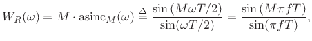
where
 |
(6.24) |
as can be seen in Fig.5.10.
Recall from §3.1.1 that the side-lobe width in a
rectangular-window transform (![]() Hz) is given in radians
per sample by
Hz) is given in radians
per sample by
 |
(6.25) |
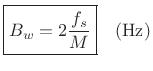
As Fig.5.10 illustrates, the rectangular-window transform main-lobe width is
|
Other Definitions of Main Lobe Width
Our simple definition of main-lobe band-width (distance between zero-crossings) works pretty well for windows in the Blackman-Harris family, which includes the first six entries in Table 5.1. (See §3.3 for more about the Blackman-Harris window family.) However, some windows have smooth transforms, such as the Hann-Poisson (Fig.3.21), or infinite-duration Gaussian window (§3.11). In particular, the true Gaussian window has a Gaussian Fourier transform, and therefore no zero crossings at all in either the time or frequency domains. In such cases, the main-lobe width is often defined using the second central moment.6.5
A practical engineering definition of main-lobe width is the minimum distance about the center such that the window-transform magnitude does not exceed the specified side-lobe level anywhere outside this interval. Such a definition always gives a smaller main-lobe width than does a definition based on zero crossings.
![\includegraphics[width=3in]{eps/windowParameters}](http://www.dsprelated.com/josimages_new/sasp2/img976.png)
In filter-design terminology, regarding the window as an FIR filter and its transform as a lowpass-filter frequency response [263], as depicted in Fig.5.11, we can say that the side lobes are everything in the stop band, while the main lobe is everything in the pass band plus the transition band of the frequency response. The pass band may be defined as some small interval about the midpoint of the main lobe. The wider the interval chosen, the larger the ``ripple'' in the pass band. The pass band can even be regarded as having zero width, in which case the main lobe consists entirely of transition band. This formulation is quite useful when designing customized windows by means of FIR filter design software, such as in Matlab or Octave (see §4.5.1, §4.10, and §3.13).
Simple Sufficient Condition for Peak Resolution
Recall from §5.4 that the frequency-domain image of a
sinusoid ``through a window'' is the window transform scaled by the
sinusoid's amplitude and shifted so that the main lobe is centered
about the sinusoid's frequency. A spectrum analysis of two sinusoids
summed together is therefore, by linearity of the Fourier transform,
the sum of two overlapping window transforms, as shown in
Fig.5.12 for the rectangular window. A simple
sufficient requirement for resolving two sinusoidal
peaks spaced ![]() Hz apart is to choose a window length long
enough so that the main lobes are clearly separated when the
sinusoidal frequencies are separated by
Hz apart is to choose a window length long
enough so that the main lobes are clearly separated when the
sinusoidal frequencies are separated by ![]() Hz. For example, we
may require that the main lobes of any Blackman-Harris window meet at
the first zero crossings in the worst case (narrowest frequency
separation); this is shown in Fig.5.12 for the rectangular-window.
Hz. For example, we
may require that the main lobes of any Blackman-Harris window meet at
the first zero crossings in the worst case (narrowest frequency
separation); this is shown in Fig.5.12 for the rectangular-window.
![\includegraphics[width=\twidth]{eps/sinesAnn}](http://www.dsprelated.com/josimages_new/sasp2/img978.png)
To obtain the separation shown in Fig.5.12, we must have
![]() Hz, where
Hz, where ![]() is the main-lobe width in Hz, and
is the main-lobe width in Hz, and
![]() is the minimum sinusoidal frequency separation in Hz.
is the minimum sinusoidal frequency separation in Hz.
For members of the ![]() -term Blackman-Harris window family,
-term Blackman-Harris window family, ![]() can
be expressed as
can
be expressed as
![]() , as indicated by
Table 5.1. In normalized radian frequency units, i.e.,
radians per sample, we have
, as indicated by
Table 5.1. In normalized radian frequency units, i.e.,
radians per sample, we have
![]() . For comparison, Table 5.2 lists minimum effective
values of
. For comparison, Table 5.2 lists minimum effective
values of ![]() for each window (denoted
for each window (denoted ![]() ) given by an
empirically verified sharper lower bound on the value needed for
accurate peak-frequency measurement [1], as discussed
further in §5.5.4 below.
) given by an
empirically verified sharper lower bound on the value needed for
accurate peak-frequency measurement [1], as discussed
further in §5.5.4 below.
|
We make the main-lobe width ![]() smaller by increasing the window
length
smaller by increasing the window
length ![]() . Specifically, requiring
. Specifically, requiring
![]() Hz implies
Hz implies
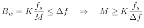 |
(6.26) |
or
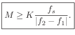
Thus, to resolve the frequencies
Periodic Signals
Many signals are periodic in nature, such as short segments of
most tonal musical instruments and speech. The sinusoidal components
in a periodic signal are constrained to be harmonic, that is,
occurring at frequencies that are an integer multiple of the
fundamental frequency ![]() .6.6 Physically, any ``driven
oscillator,'' such as bowed-string instruments, brasses, woodwinds,
flutes, etc., is usually quite periodic in normal steady-state
operation, and therefore generates harmonic overtones in steady
state. Freely vibrating resonators, on the other hand, such as
plucked strings, gongs, and ``tonal percussion'' instruments,
are not generally periodic.6.7
.6.6 Physically, any ``driven
oscillator,'' such as bowed-string instruments, brasses, woodwinds,
flutes, etc., is usually quite periodic in normal steady-state
operation, and therefore generates harmonic overtones in steady
state. Freely vibrating resonators, on the other hand, such as
plucked strings, gongs, and ``tonal percussion'' instruments,
are not generally periodic.6.7
Consider a periodic signal with fundamental frequency ![]() Hz.
Then the harmonic components occur at integer multiples of
Hz.
Then the harmonic components occur at integer multiples of ![]() , and
so they are spaced in frequency by
, and
so they are spaced in frequency by
![]() . To resolve
these harmonics in a spectrum analysis, we require, adapting
(5.27),
. To resolve
these harmonics in a spectrum analysis, we require, adapting
(5.27),
 |
(6.28) |
Note that
 is the fundamental period of the signal in samples.
Thus, another way of stating our simple, sufficient resolution
requirement on window length
is the fundamental period of the signal in samples.
Thus, another way of stating our simple, sufficient resolution
requirement on window length
Specifically, resolving the harmonics of a periodic signal with period
![]() samples is assured if we have at least
samples is assured if we have at least
 periods under the rectangular window,
 periods under the Hamming window,
 periods under the Blackman window,
 periods under the Blackman-Harris
  -term window,
![\begin{figure*}\centering
\subfigure[Length $M=100$\ rectangular window]{
\epsfxsize =\twidth
\epsfysize =1.5in \epsfbox{eps/EffectiveLength1.eps}
}
\subfigure[Length $M=200$\ Hamming window]{
\epsfxsize =\twidth
\epsfysize =1.5in \epsfbox{eps/EffectiveLength2.eps}
}
\subfigure[Length $M=300$\ Blackman window]{
\epsfxsize =\twidth
\epsfysize =1.5in \epsfbox{eps/EffectiveLength3.eps}
}\end{figure*}](http://www.dsprelated.com/josimages_new/sasp2/img1005.png) |
Tighter Bounds for Minimum Window Length
[This section, adapted from [1], is relatively advanced and may be skipped without loss of continuity.]
Figures 5.14(a) through 5.14(d) show four possible definitions of main-lobe separation that could be considered for purposes of resolving closely spaced sinusoidal peaks.
![\begin{figure*}\centering
\subfigure[Minimum orthogonal separation]{
\epsfxsize =4.0in
\epsfysize =1.0in \epsfbox{eps/SpecResCases1.eps}
}
\subfigure[Separation to first stationary-point \cite{AbeAndSmith04}]{
\epsfxsize =4.0in
\epsfysize =1.0in \epsfbox{eps/SpecResCases2.eps}
}
\subfigure[Separation to where main-lobe level equals side-lobe level]{
\epsfxsize =4.0in
\epsfysize =1.0in \epsfbox{eps/SpecResCases3.eps}
}
\subfigure[Full main-lobe separation]{
\epsfxsize =4.0in
\epsfysize =1.0in \epsfbox{eps/SpecResCases4.eps}
}\end{figure*}](http://www.dsprelated.com/josimages_new/sasp2/img1006.png) |
In Fig.5.14(a), the main lobes sit atop each other's first zero
crossing. We may call this the ``minimum orthogonal separation,'' so
named because we know from Discrete Fourier Transform theory
[264] that ![]() -sample segments of sinusoids at this
frequency-spacing are exactly orthogonal. (
-sample segments of sinusoids at this
frequency-spacing are exactly orthogonal. (![]() is the
rectangular-window length as before.) At this spacing, the peak of
each main lobe is unchanged by the ``interfering'' window transform.
However, the slope and higher derivatives at each peak
are modified by the presence of the interfering window
transform. In practice, we must work over a discrete frequency axis,
and we do not, in general, sample exactly at each main-lobe peak.
Instead, we usually determine an interpolated peak location
based on samples near the true peak location. For example, quadratic
interpolation, which is commonly used, requires at least three samples
about each peak (as discussed in §5.7 below), and it is
therefore sensitive to a nonzero slope at the peak. Thus, while
minimum-orthogonal spacing is ideal in the limit as the sampling
density along the frequency axis approaches infinity, it is not ideal
in practice, even when we know the peak frequency-spacing
exactly.6.8
is the
rectangular-window length as before.) At this spacing, the peak of
each main lobe is unchanged by the ``interfering'' window transform.
However, the slope and higher derivatives at each peak
are modified by the presence of the interfering window
transform. In practice, we must work over a discrete frequency axis,
and we do not, in general, sample exactly at each main-lobe peak.
Instead, we usually determine an interpolated peak location
based on samples near the true peak location. For example, quadratic
interpolation, which is commonly used, requires at least three samples
about each peak (as discussed in §5.7 below), and it is
therefore sensitive to a nonzero slope at the peak. Thus, while
minimum-orthogonal spacing is ideal in the limit as the sampling
density along the frequency axis approaches infinity, it is not ideal
in practice, even when we know the peak frequency-spacing
exactly.6.8
Figure 5.14(b) shows the ``zero-error stationary point'' frequency
spacing. In this case, the main-lobe peak of one
![]() sits atop
the first local minimum from the main-lobe of the other
sits atop
the first local minimum from the main-lobe of the other
![]() . Since the derivative of both
. Since the derivative of both
![]() functions is zero at
both peak frequencies at this spacing, the peaks do not ``sit on a
slope'' which would cause the peak locations to be biased away
from the sinusoidal frequencies. We may say that peak-frequency
estimates based on samples about the peak will be unbiased, to first
order, at this spacing. This minimum spacing, which is easy to
compute for Blackman-Harris windows, turns out to be very close to the
optimal minimum spacing [1].
functions is zero at
both peak frequencies at this spacing, the peaks do not ``sit on a
slope'' which would cause the peak locations to be biased away
from the sinusoidal frequencies. We may say that peak-frequency
estimates based on samples about the peak will be unbiased, to first
order, at this spacing. This minimum spacing, which is easy to
compute for Blackman-Harris windows, turns out to be very close to the
optimal minimum spacing [1].
Figure 5.14(c) shows the minimum frequency spacing which naturally matches side-lobe level. That is, the main lobes are pulled apart until the main-lobe level equals the worst-case side-lobe level. This spacing is usually not easy to compute, and it is best matched with the Chebyshev window (see §3.10). Note that it is just a little wider than the stationary-point spacing discussed in the previous paragraph.
For ease of comparison, Fig.5.14(d) shows once again the simple, sufficient rule (''full main-lobe separation'') discussed in §5.5.2 above. While overly conservative, it is easily computed for many window types (any window with a known main-lobe width), and so it remains a useful rule-of-thumb for determining minimum window length given the minimum expected frequency spacing.
A table of minimum window lengths for the Kaiser window, as a function of frequency spacing, is given in §3.9.
Summary
We see that when measuring sinusoidal peaks, it is important to know the minimum frequency separation of the peaks, and to choose an FFT window which is long enough to resolve the peaks accurately. Generally speaking, the window must ``see'' at least 1.5 cycles of the minimum difference frequency. The rectangular window ``sees'' its full length. Other windows, which are all tapered in some way (Chapter 3), see an effective duration less than the window length in samples. Further details regarding theoretical and empirical estimates are given in [1].
Next Section:
Sinusoidal Peak Interpolation
Previous Section:
Effect of Windowing


