Sinusoidal Peak Interpolation

Free Books Spectral Audio Signal Processing

In §2.5, we discussed ideal spectral interpolation (zero-padding in the time domain followed by an FFT). Since FFTs are efficient, this is an efficient interpolation method. However, in audio spectral modeling, there is usually a limit on the needed accuracy due to the limitations of audio perception. As a result, a ``perceptually ideal'' spectral interpolation method that is even more efficient is to zero-pad by some small factor (usually less than 5), followed by quadratic interpolation of the spectral magnitude. We call this the quadratically interpolated FFT (QIFFT) method [271,1]. The QIFFT method is usually more efficient than the equivalent degree of ideal interpolation, for a given level of perceptual error tolerance (specific guidelines are given in §5.6.2 below). The QIFFT method can be considered an approximate maximum likelihood method for spectral peak estimation, as we will see.

Quadratic Interpolation of Spectral Peaks

In quadratic interpolation of sinusoidal spectrum-analysis peaks, we replace the main lobe of our window transform by a quadratic polynomial, or ``parabola''. This is valid for any practical window transform in a sufficiently small neighborhood about the peak, because the higher order terms in a Taylor series expansion about the peak converge to zero as the peak is approached.

Note that, as mentioned in §D.1, the Gaussian window transform magnitude is precisely a parabola on a dB scale. As a result, quadratic spectral peak interpolation is exact under the Gaussian window. Of course, we must somehow remove the infinitely long tails of the Gaussian window in practice, but this does not cause much deviation from a parabola, as shown in Fig.3.36.

$\begin{psfrags} % latex2html id marker 16827\psfrag{a} []{ \Large$ \alpha $}\psfrag{b} []{ \Large$ \beta $}\psfrag{g} []{ \Large$ \gamma $\ }\begin{figure}[htbp] \includegraphics[width=\textwidth ]{eps/parabola} \caption{Illustration of parabolic peak interpolation using the three samples nearest the peak.} \end{figure} \end{psfrags}$

Referring to Fig.5.15, the general formula for a parabola may be written as

$\displaystyle y(x) \mathrel{\stackrel{\Delta}{=}}a(x-p)^2+b$

(6.29)

The center point gives us our interpolated peak location (in bins), while the amplitude equals the peak amplitude (typically in dB). The curvature depends on the window used and contains no information about the sinusoid. (It may, however, indicate that the peak being interpolated is not a pure sinusoid.)

At the three samples nearest the peak, we have

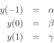
$\begin{eqnarray*} y(-1) &=& \alpha \\ y(0) &=& \beta \\ y(1) &=& \gamma \end{eqnarray*}$

where we arbitrarily renumbered the bins about the peak , 0, and 1. Writing the three samples in terms of the interpolating parabola gives

$\begin{eqnarray*} \alpha &=& ap^2 + 2ap + a + b \\ \beta &=& ap^2 + b \\ \gamma &=& ap^2 - 2ap + a + b \end{eqnarray*}$

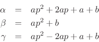
which implies

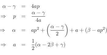
$\begin{eqnarray*} \alpha- \gamma &=& 4ap \\ \Rightarrow\quad p &=& \frac{\alpha-\gamma}{4a} \\ \Rightarrow\quad \alpha &=& ap^2 + \left(\frac{\alpha-\gamma}{2}\right) +a+(\beta-ap^2) \\ \Rightarrow\quad a &=& \frac{1}{2}(\alpha - 2\beta + \gamma) \\ \end{eqnarray*}$

Hence, the interpolated peak location is given in bins^6.9 (spectral samples) by

$\displaystyle \zbox {p=\frac{1}{2}\frac{\alpha-\gamma}{\alpha-2\beta+\gamma}} \in [-1/2,1/2].$

(6.30)

If $k^\ast$ denotes the bin number of the largest spectral sample at the peak, then $k^\ast+p$ is the interpolated peak location in bins. The final interpolated frequency estimate is then $(k^\ast+p)f_s/N$ Hz, where denotes the sampling rate and is the FFT size.

Using the interpolated peak location, the peak magnitude estimate is

$\displaystyle \zbox {y(p) = \beta - \frac{1}{4}(\alpha-\gamma)p.}$

(6.31)

Phase Interpolation at a Peak

Note that only the spectral magnitude is used to find in the parabolic interpolation scheme of the previous section. In some applications, a phase interpolation is also desired.

In principle, phase interpolation is independent of magnitude interpolation, and any interpolation method can be used. There is usually no reason to expect a ``phase peak'' at a magnitude peak, so simple linear interpolation may be used to interpolate the unwrapped phase samples (given a sufficiently large zero-padding factor). Matlab has an unwrap function for unwrapping phase, and §F.4 provides an Octave-compatible version.

If we do expect a phase peak (such as when identifying chirps, as discussed in §10.6), then we may use quadratic interpolation separately on the (unwrapped) phase.

Alternatively, the real and imaginary parts can be interpolated separately to yield a complex peak value estimate.

Matlab for Parabolic Peak Interpolation

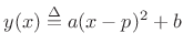
Section §F.2 lists Matlab/Octave code for finding quadratically interpolated peaks in the magnitude spectrum as discussed above. At the heart is the qint function, which contains the following:

function [p,y,a] = qint(ym1,y0,yp1)
%QINT - quadratic interpolation of three adjacent samples
%
% [p,y,a] = qint(ym1,y0,yp1)
%
% returns the extremum location p, height y, and half-curvature a
% of a parabolic fit through three points.
% Parabola is given by y(x) = a*(x-p)^2+b,
% where y(-1)=ym1, y(0)=y0, y(1)=yp1.

p = (yp1 - ym1)/(2*(2*y0 - yp1 - ym1));
y = y0 - 0.25*(ym1-yp1)*p;
a = 0.5*(ym1 - 2*y0 + yp1);

Bias of Parabolic Peak Interpolation

Since the true window transform is not a parabola (except for the conceptual case of a Gaussian window transform expressed in dB), there is generally some error in the interpolated peak due to this mismatch. Such a systematic error in an estimated quantity (due to modeling error, not noise), is often called a bias. Parabolic interpolation is unbiased when the peak occurs at a spectral sample (FFT bin frequency), and also when the peak is exactly half-way between spectral samples (due to symmetry of the window transform about its midpoint). For other peak frequencies, quadratic interpolation yields a biased estimate of both peak frequency and peak amplitude. (Phase is essentially unbiased [1].)

Since zero-padding in the time domain gives ideal interpolation in the frequency domain, there is no bias introduced by this type of interpolation. Thus, if enough zero-padding is used so that a spectral sample appears at the peak frequency, simply finding the largest-magnitude spectral sample will give an unbiased peak-frequency estimator. (We will learn in §5.7.2 that this is also the maximum likelihood estimator for the frequency of a sinusoid in additive white Gaussian noise.)

While we could choose our zero-padding factor large enough to yield any desired degree of accuracy in peak frequency measurements, it is more efficient in practice to combine zero-padding with parabolic interpolation (or some other simple, low-order interpolator). In such hybrid schemes, the zero-padding is simply chosen large enough so that the bias due to parabolic interpolation is negligible. In §5.7 below, the Quadratically Interpolated FFT (QIFFT) method is described as one such hybrid scheme.

Next Section:
Optimal Peak-Finding in the Spectrum
Previous Section:
Resolving Sinusoids