Spectral Modeling Synthesis

Free Books Spectral Audio Signal Processing

This section reviews elementary spectral models for sound synthesis. Spectral models are well matched to audio perception because the ear is a kind of spectrum analyzer [293].

For periodic sounds, the component sinusoids are all harmonics of a fundamental at frequency $\omega_1$ :

$\displaystyle s(t) = \sum_{k=0}^K A_k \sin(\omega_k t + \phi_k) \protect$

(11.15)

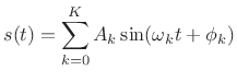
where denotes time in seconds, $\omega_k = k\cdot 2\pi/P$ is the th harmonic radian frequency, is the period in seconds, is the amplitude of the th sinusoidal component, $\phi_k$ is its phase, and is the number of the highest audible harmonic.

Aperiodic sounds can similarly be expressed as a continuous sum of sinusoids at potentially all frequencies in the range of human hearing:^11.6

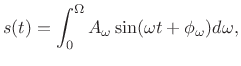
$\displaystyle s(t) = \int_{0}^\Omega A_\omega \sin(\omega t + \phi_\omega) d\omega, \protect$

(11.16)

where $\Omega$ denotes the upper bound of human hearing (nominally $2\pi\cdot 20$ kHz).

Sinusoidal models are most appropriate for ``tonal'' sounds such as spoken or sung vowels, or the sounds of musical instruments in the string, wind, brass, and ``tonal percussion'' families. Ideally, one sinusoid suffices to represent each harmonic or overtone.^11.7 To represent the ``attack'' and ``decay'' of natural tones, sinusoidal components are multiplied by an amplitude envelope that varies over time. That is, the amplitude in (10.15) is a slowly varying function of time; similarly, to allow pitch variations such as vibrato, the phase $\phi_k(t)$ may be modulated in various ways.^11.8 Sums of amplitude- and/or frequency-enveloped sinusoids are generally called additive synthesis (discussed further in §10.4.1 below).

Sinusoidal models are ``unreasonably effective'' for tonal audio. Perhaps the main reason is that the ear focuses most acutely on peaks in the spectrum of a sound [179,305]. For example, when there is a strong spectral peak at a particular frequency, it tends to mask lower level sound energy at nearby frequencies. As a result, the ear-brain system is, to a first approximation, a ``spectral peak analyzer''. In modern audio coders [16,200] exploiting masking results in an order-of-magnitude data compression, on average, with no loss of quality, according to listening tests [25]. Thus, we may say more specifically that, to first order, the ear-brain system acts like a ``top ten percent spectral peak analyzer''.

For noise-like sounds, such as wind, scraping sounds, unvoiced speech, or breath-noise in a flute, sinusoidal models are relatively expensive, requiring many sinusoids across the audio band to model noise. It is therefore helpful to combine a sinusoidal model with some kind of noise model, such as pseudo-random numbers passed through a filter [249]. The ``Sines + Noise'' (S+N) model was developed to use filtered noise as a replacement for many sinusoids when modeling noise (to be discussed in §10.4.3 below).

Another situation in which sinusoidal models are inefficient is at sudden time-domain transients in a sound, such as percussive note onsets, ``glitchy'' sounds, or ``attacks'' of instrument tones more generally. From Fourier theory, we know that transients, too, can be modeled exactly, but only with large numbers of sinusoids at exactly the right phases and amplitudes. To obtain a more compact signal model, it is better to introduce an explicit transient model which works together with sinusoids and filtered noise to represent the sound more parsimoniously. Sines + Noise + Transients (S+N+T) models were developed to separately handle transients (§10.4.4).

A advantage of the explicit transient model in S+N+T models is that transients can be preserved during time-compression or expansion. That is, when a sound is stretched (without altering its pitch), it is usually desirable to preserve the transients (i.e., to keep their local time scales unchanged) and simply translate them to new times. This topic, known as Time-Scale Modification (TSM) will be considered further in §10.5 below.

In addition to S+N+T components, it is useful to superimpose spectral weightings to implement linear filtering directly in the frequency domain; for example, the formants of the human voice are conveniently impressed on the spectrum in this way (as illustrated §10.3 above) [174].^11.9 We refer to the general class of such frequency-domain signal models as spectral models, and sound synthesis in terms of spectral models is often called spectral modeling synthesis (SMS).

The subsections below provide a summary review of selected aspects of spectral modeling, with emphasis on applications in musical sound synthesis and effects.

Additive Synthesis (Early Sinusoidal Modeling)

Additive synthesis is evidently the first technique widely used for analysis and synthesis of audio in computer music [232,233,184,186,187]. It was inspired directly by Fourier theory [264,23,36,150] (which followed Daniel Bernoulli's insights (§G.1)) which states that any sound can be expressed mathematically as a sum of sinusoids. The `term ``additive synthesis'' refers to sound being formed by adding together many sinusoidal components modulated by relatively slowly varying amplitude and frequency envelopes:

$\displaystyle y(t)= \sum\limits_{i=1}^{N} A_i(t)\sin[\theta_i(t)]$

(11.17)

where

$\displaystyle A_i(t)$	$\displaystyle =$	$\displaystyle \hbox{amplitude of $i$th partial over time $t$}$
$\displaystyle \theta_i(t)$	$\displaystyle =$	$\displaystyle \int_0^t \omega_i(t)dt + \phi_i(0)$
$\displaystyle \omega_i(t)$	$\displaystyle =$	$\displaystyle d\theta_i(t)/dt = \hbox{radian frequency of $i$th partial vs.\ time}$
$\displaystyle \phi_i(0)$	$\displaystyle =$	$\displaystyle \hbox{phase offset of $i$th partial at time $0$} \protect$	(11.18)

and all quantities are real. Thus, each sinusoid may have an independently time-varying amplitude and/or phase, in general. The amplitude and frequency envelopes are determined from some kind of short-time Fourier analysis as discussed in Chapters 8 and 9) [62,187,184,186].

An additive-synthesis oscillator-bank is shown in Fig.10.7, as it is often drawn in computer music [235,234]. Each sinusoidal oscillator [166] accepts an amplitude envelope (e.g., piecewise linear, or piecewise exponential) and a frequency envelope , also typically piecewise linear or exponential. Also shown in Fig.10.7 is a filtered noise input, as used in S+N modeling (§10.4.3).

$\begin{psfrags} % latex2html id marker 27324\psfrag{A1} []{ \Large$ A_1(t)$\ }\psfrag{A2} []{ \Large$ A_2(t)$\ }\psfrag{A3} []{ \Large$ A_3(t)$\ }\psfrag{A4} []{ \Large$ A_4(t)$\ }\psfrag{f1} []{ \Large$ f_1(t)$\ }\psfrag{f2} []{ \Large$ f_2(t)$\ }\psfrag{f3} []{ \Large$ f_3(t)$\ }\psfrag{f4} []{ \Large$ f_4(t)$\ }\psfrag{s} [b]{ {\Huge$\sum$} }\psfrag{noise} [][b]{{\Large$\stackrel{\hbox{[new] noise}}{u(t)}$}}\psfrag{Filter} [][c]{{\Large$\stackrel{\hbox{filter}}{h_t(\tau)}$}}\psfrag{out} []{ {\large$ y(t)= \sum\limits_{i=1}^{4} A_i(t)\sin\left[\int_0^t\omega_i(t)dt +\phi_i(0)\right] + (h_t \ast u)(t) $\ = sine-sum + filtered-noise}}\begin{figure}[htbp] \includegraphics[width=0.9\twidth]{eps/additive} \caption{Sinusoidal oscillator bank and filtered noise for sines+noise spectral modeling synthesis.} \end{figure} \end{psfrags}$

Additive Synthesis Analysis

In order to reproduce a given signal, we must first analyze it to determine the amplitude and frequency trajectories for each sinusoidal component. We do not need phase information ( $\phi_i$ in (10.18)) during steady-state segments, since phase is normally not perceived in steady state tones [293,211]. However, we do need phase information for analysis frames containing an attack transient, or any other abrupt change in the signal. The phase of the sinusoidal peaks controls the position of time-domain features of the waveform within the analysis frame.

Following Spectral Peaks

In the analysis phase, sinusoidal peaks are measured over time in a sequence of FFTs, and these peaks are grouped into ``tracks'' across time. A detailed discussion of various options for this can be found in [246,174,271,84,248,223,10,146], and a particular case is detailed in Appendix H.

The end result of the analysis pass is a collection of amplitude and frequency envelopes for each spectral peak versus time. If the time advance from one FFT to the next is fixed (5ms is a typical choice for speech analysis), then we obtain uniformly sampled amplitude and frequency trajectories as the result of the analysis. The sampling rate of these amplitude and frequency envelopes is equal to the frame rate of the analysis. (If the time advance between FFTs is $\Delta t=5$ ms, then the frame rate is defined as $1/\Delta t = 200$ Hz.) For resynthesis using inverse FFTs, these data may be used unmodified. For resynthesis using a bank of sinusoidal oscillators, on the other hand, we must somehow interpolate the envelopes to create envelopes at the signal sampling rate (typically kHz or higher).

It is typical in computer music to linearly interpolate the amplitude and frequency trajectories from one frame to the next [271].^11.10 Let's call the piecewise-linear upsampled envelopes ${\hat A}_k(n)$ and $\hat{F}_k(n)$ , defined now for all at the normal signal sampling rate. For steady-state tonal sounds, the phase may be discarded at this stage and redefined as the integral of the instantaneous frequency when needed:

$\displaystyle \hat{\Theta }_k(n) \isdefs \hat{\Theta }_k(n-1) + 2\pi T \hat{F}_k(n). \protect$

(11.19)

When phase must be matched in a given frame, such as when it is known to contain a transient event, the frequency can instead move quadratically across the frame to provide cubic phase interpolation [174], or a second linear breakpoint can be introduced somewhere in the frame for the frequency trajectory (in which case the area under the triangle formed by the second breakpoint equals the added phase at the end of the segment).

Sinusoidal Peak Finding

For each sinusoidal component of a signal, we need to determine its frequency, amplitude, and phase (when needed). As a starting point, consider the windowed complex sinusoid with complex amplitude ${\cal A}_x$ and frequency $\omega _x$ :

$\displaystyle x_w(n) = w(n){\cal A}_xe^{j\omega_x nT}$

(11.20)

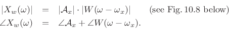
As discussed in Chapter 5, the transform (DTFT) of this windowed signal is the convolution of a frequency domain delta function at $\omega _x$ [ $\delta(\omega - \omega_x)$ ], and the transform of the window function, $W(\omega)$ , resulting in a shifted version of the window transform ${\cal A}_xW(\omega-\omega_x)$ . Assuming is odd, we can show this as follows:

$\begin{eqnarray*} X_w(\omega) &=& \sum_{n=-\infty}^{\infty}[w(n)x(n)]e^{ -j\omega nT} \qquad\hbox{(DTFT($x_w$))} \\ &=& \sum_{n=-(M-1)/2}^{(M-1)/2} \left[w(n){\cal A}_xe^{j\omega_xnT}\right]e^{ -j\omega nT}\\ &=& {\cal A}_x\sum_n w(n) e^{-j(\omega-\omega_x)nT} \\ &=& \zbox {{\cal A}_xW(\omega-\omega_x)} \end{eqnarray*}$

Hence,

$\begin{eqnarray*} \vert X_w(\omega) \vert &=& \vert{\cal A}_x\vert \cdot \vert W(\omega-\omega_x)\vert \qquad \hbox{(see \fref {peak} below)}\\ \angle X_w(\omega) &=& \angle {\cal A}_x+ \angle W(\omega-\omega_x). \end{eqnarray*}$

At $\omega _x$ , we have

$\begin{eqnarray*} \vert X_w(\omega_x)\vert &=& \vert{\cal A}_x\vert\cdot \vert W(0)\vert \\ \angle X_w(\omega_x)\vert &=& \angle {\cal A}_x+ \angle W(0) \end{eqnarray*}$

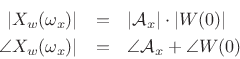
If we scale the window to have a dc gain of 1, then the peak magnitude equals the amplitude of the sinusoid, i.e., 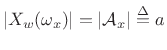$\vert X_w(\omega_x)\vert=\vert{\cal A}_x\vert\isdef a$ , as shown in Fig.10.8.

**Figure:** Schematic diagram of a window transform amplitude-scaled by and frequency-shifted by **$\omega _x$** .
$\includegraphics[width=0.8\twidth]{eps/peak}$

If we use a zero-phase (even) window, the phase at the peak equals the phase of the sinusoid, i.e., $\angle X_w(\omega_x) = \angle {\cal A}_x$ .

Tracking Sinusoidal Peaks in a Sequence of FFTs

The preceding discussion focused on estimating sinusoidal peaks in a single frame of data. For estimating sinusoidal parameter trajectories through time, it is necessary to associate peaks from one frame to the next. For example, Fig.10.9 illustrates a set of frequency trajectories, including one with a missing segment due to its peak not being detected in the third frame.

**Figure 10.9:** Sinusoidal frequency trajectories.
$\includegraphics[width=0.8\twidth]{eps/tracks}$

Figure 10.10 depicts a basic analysis system for tracking spectral peaks in the STFT [271]. The system tracks peak amplitude, center-frequency, and sometimes phase. Quadratic interpolation is used to accurately find spectral magnitude peaks (§5.7). For further analysis details, see Appendix H. Synthesis is performed using a bank of amplitude- and phase-modulated oscillators, as shown in Fig.10.7. Alternatively, the sinusoids are synthesized using an inverse FFT [239,94,139].

$\begin{psfrags} % latex2html id marker 27619\psfrag{s} []{\Large$s(t)$}\psfrag{tan} []{\Large$\tan^{-1}$}\begin{figure}[htbp] \includegraphics[width=\twidth]{eps/analysis} \caption{Block diagram of a sinusoidal-modeling \emph{analysis} system (from \cite{SerraT}).} \end{figure} \end{psfrags}$

Sines + Noise Modeling

As mentioned in the introduction to this chapter, it takes many sinusoidal components to synthesize noise well (as many as 25 per critical band of hearing under certain conditions [85]). When spectral peaks are that dense, they are no longer perceived individually, and it suffices to match only their statistics to a perceptually equivalent degree.

Sines+Noise (S+N) synthesis [249] generalizes the sinusoidal signal models to include a filtered noise component, as depicted in Fig.10.7. In that figure, white noise is denoted by , and the slowly changing linear filter applied to the noise at time is denoted $h_t(\cdot)$ .

The time-varying spectrum of the signal is said to be made up of a deterministic component (the sinusoids) and a stochastic component (time-varying filtered noise) [246,249]:

$\displaystyle s(t) \eqsp \sum_{i=1}^{N} A_i(t) \cos[ \theta_i(t)] + e(t),$

(11.21)

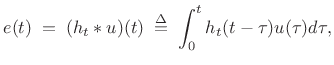where and $\theta_i(t)$ are the instantaneous amplitude and phase of the th sinusoidal component, and is the residual, or noise signal, assumed to be well modeled by filtered white noise:

$\displaystyle e(t) \eqsp (h_t \ast u)(t) \isdefs \int_0^t h_{t}(t-\tau)u(\tau)d\tau,$

(11.22)

where is the white noise, and $h_t(\tau)$ is the impulse response of a time varying linear filter at time . Specifically, $h_t(\tau)$ is the response at time to an impulse at time $t-\tau$ .

Filtering white-noise to produce a desired timbre is an example of subtractive synthesis [186]. Thus, additive synthesis is nicely supplemented by subtractive synthesis as well.

Sines+Noise Analysis

The original sines+noise analysis method is shown in Fig.10.11 [246,249]. The processing path along the top from left to right measures the amplitude and frequency trajectories from magnitude peaks in the STFT, as in Fig.10.10. The peak amplitude and frequency trajectories are converted back to the time domain by additive-synthesis (an oscillator bank or inverse FFT), and this signal is windowed by the same analysis window and forward-transformed back into the frequency domain. The magnitude-spectrum of this sines-only data is then subtracted from the originally computed magnitude-spectrum containing both peaks and ``noise''. The result of this subtraction is termed the residual signal. The upper spectral envelope of the residual magnitude spectrum is measured using, e.g., linear prediction, cepstral smoothing, as discussed in §10.3 above, or by simply connecting peaks of the residual spectrum with linear segments to form a more traditional (in computer music) piecewise linear spectral envelope.

$\begin{psfrags} % latex2html id marker 27835\psfrag{s}{\Large $x(n)$}\begin{figure}[htbp] \includegraphics[width=\twidth]{eps/smsanal} \caption{Sines+noise analysis diagram (from \cite{SerraT}).} \end{figure} \end{psfrags}$

S+N Synthesis

A sines+noise synthesis diagram is shown in Fig.10.12. The spectral-peak amplitude and frequency trajectories are possibly modified (time-scaling, frequency scaling, virtual formants, etc.) and then rendered into the time domain by additive synthesis. This is termed the deterministic part of the synthesized signal.

The stochastic part is synthesized by applying the residual-spectrum-envelope (a time-varying FIR filter) to white noise, again after possible modifications to the envelope.

To synthesize a frame of filtered white noise, one can simply impart a random phase to the spectral envelope, i.e., multiply it by $\exp[j\phi(\omega_k)]$ , where $\phi(\omega_k)$ is random and uniformly distributed between $-\pi$ and $\pi$ . In the time domain, the synthesized white noise will be approximately Gaussian due to the central limit theorem (§D.9.1). Because the filter (spectral envelope) is changing from frame to frame through time, it is important to use at least 50% overlap and non-rectangular windowing in the time domain. The window can be implemented directly in the frequency domain by convolving its transform with the complex white-noise spectrum (§3.3.5), leaving only overlap-add to be carried out in the time domain. If the window side-lobes can be fully neglected, it suffices to use only main lobe in such a convolution [239].

In Fig.10.12, the deterministic and stochastic components are summed after transforming to the time domain, and this is the typical choice when an explicit oscillator bank is used for the additive synthesis. When the IFFT method is used for sinusoid synthesis [239,94,139], the sum can occur in the frequency domain, so that only one inverse FFT is required.

$\begin{psfrags} % latex2html id marker 27855\psfrag{IFFT} [][c]{{\Large IFFT $\cdot w$}}\begin{figure}[htbp] \includegraphics[width=\twidth]{eps/smssynth} \caption{Sines+noise synthesis diagram (from \cite{SerraT}).} \end{figure} \end{psfrags}$

Sines+Noise Summary

To summarize, sines+noise modeling is carried out by a procedure such as the following:

Compute a sinusoidal model by tracking peaks across STFT frames, producing a set of amplitude envelopes and frequency envelopes , where is the frame number and is the spectral-peak number.
Also record phase $\Theta_m(\omega_k)$ for frames containing a transient.
Subtract modeled peaks from each STFT spectrum to form a residual spectrum.
Fit a smooth spectral envelope $H_m(\omega_k)$ to each residual spectrum.
Convert envelopes to reduced form, e.g., piecewise linear segments with nonuniformly distributed breakpoints (optimized to be maximally sparse without introducing audible distortion).
Resynthesize audio (along with any desired transformations) from the amplitude, frequency, and noise-floor-filter envelopes.
Alter frequency trajectories slightly to hit the desired phase for transient frames (as described below equation Eq. $\,$ (10.19)).

Because the signal model consists entirely of envelopes (neglecting the phase data for transient frames), the signal model is easily time scaled, as discussed further in §10.5 below.

For more information on sines+noise signal modeling, see, e.g., [146,10,223,248,246,149,271,248,271]. A discussion from an historical perspective appears in §G.11.4.

Sines + Noise + Transients Models

As we have seen, sinusoids efficiently model spectral peaks over time, and filtered noise efficiently models the spectral residual left over after pulling out everything we want to call a ``tonal component'' characterized by a spectral peak the evolves over time. However, neither is good for abrupt transients in a waveform. At transients, one may retain the original waveform or some compressed version of it (e.g., MPEG-2 AAC with short window [149]). Alternatively, one may switch to a transient model during transients. Transient models have included wavelet expansion [6] and frequency-domain LPC (time-domain amplitude envelope) [290].

In either case, a reliable transient detector is needed. This can raise deep questions regarding what a transient really is; for example, not everyone will notice every transient as a transient, and so perceptual modeling gets involved. Missing a transient, e.g., in a ride-cymbal analysis, can create highly audible artifacts when processing heavily based on transient decisions. For greater robustness, hybrid schemes can be devised in which a continuous measure of ``transientness'' ${\cal T}$ can be defined between 0 and 1, say.

Also in either case, the sinusoidal model needs phase matching when switching to or from a transient frame over time (or cross-fading can be used, or both). Given sufficiently many sinusoids, phase-matching at the switching time should be sufficient without cross-fading.

Sines+Noise+Transients Time-Frequency Maps

Figure 10.13 shows the multiresolution time-frequency map used in the original S+N+T system [149]. (Recall the fixed-resolution STFT time-frequency map in Fig.7.1.) Vertical line spacing in the time-frequency map indicates the time resolution of the underlying multiresolution STFT,^11.11 and the horizontal line spacing indicates its frequency resolution. The time waveform appears below the time-frequency map. For transients, an interval of data including the transient is simply encoded using MPEG-2 AAC. The transient-time in Fig.10.13 extends from approximately 47 to 115 ms. (This interval can be tighter, as discussed further below.) Between transients, the signal model consists of sines+noise below 5 kHz and amplitude-modulated noise above. The spectrum from 0 to 5 kHz is divided into three octaves (``multiresolution sinusoidal modeling''). The time step-size varies from 25 ms in the low-frequency band (where the frequency resolution is highest), down to 6 ms in the third octave (where frequency resolution is four times lower). In the 0-5 kHz band, sines+noise modeling is carried out. Above 5 kHz, noise substitution is performed, as discussed further below.

**Figure 10.13:** S+N+T Time-Frequency Map (from [149]).
$\includegraphics[width=0.9\twidth]{eps/scottl-tf-aac}$

Figure 10.14 shows a similar map in which the transient interval depends on frequency. This enables a tighter interval enclosing the transient, and follows audio perception more closely (see Appendix E).

**Figure 10.14:** Quasi-Constant-Q (Wavelet) Time-Frequency Map [149].
$\includegraphics[width=0.9\twidth]{eps/scottl-tf-smooth}$

Sines+Noise+Transients Noise Model

Figure 10.15 illustrates the nature of the noise modeling used in [149]. The energy in each Bark band ^11.12 is summed, and this is used as the gain for the noise in that band at that frame time.

**Figure 10.15:** Bark-band noise modeling (from [149]).
$\includegraphics[width=0.9\twidth]{eps/scottl-bark-noise}$

Figure 10.16 shows the frame gain versus time for a particular Bark band (top) and the piecewise linear envelope made from it (bottom). As illustrated in Figures 10.13 and 10.14, the step size for all of the Bark bands above 5 kHz is approximately 3 ms.

**Figure 10.16:** Amplitude envelope for one noise band (from [149]).
$\includegraphics[width=0.9\twidth]{eps/scottl-noise-env}$

S+N+T Sound Examples

A collection of sound examples illustrating sines+noise+transients modeling (and various subsets thereof) as well as some audio effects made possible by such representations, can be found online at
http://ccrma.stanford.edu/~jos/pdf/SMS.pdf.

Discussion regarding S+N+T models in historical context is given in §G.11.5.

Next Section:
Time Scale Modification
Previous Section:
Spectral Envelope Extraction