


Summary of LP Spectral Envelopes
In summary, the spectral envelope of the ![]() th spectral frame,
computed by linear prediction, is given by
th spectral frame,
computed by linear prediction, is given by
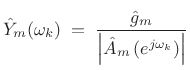 |
(11.13) |
where
 |
(11.14) |
can be driven by unit-variance white noise to produce a filtered-white-noise signal having spectral envelope
It bears repeating that
![]() is zero mean when
is zero mean when
![]() is monic and minimum phase (all zeros inside the unit circle).
This means, for example, that
is monic and minimum phase (all zeros inside the unit circle).
This means, for example, that
![]() can be simply estimated as
the mean of the log spectral magnitude
can be simply estimated as
the mean of the log spectral magnitude
![]() .
.
For best results, the frequency axis ``seen'' by linear prediction should be warped to an auditory frequency scale, as discussed in Appendix E [123]. This has the effect of increasing the accuracy of low-frequency peaks in the extracted spectral envelope, in accordance with the nonuniform frequency resolution of the inner ear.
Next Section:
Signal Synthesis
Previous Section:
Linear Prediction Order Selection


