


Synthesis (Step 7)
The analysis portion of PARSHL returns a set of amplitudes
![]() , frequencies
, frequencies
![]() , and phases
, and phases
![]() ,
for each frame index
,
for each frame index ![]() , with a ``triad'' (
, with a ``triad'' (
![]() ) for each track
) for each track ![]() . From this analysis data the
program has the option of generating a synthetic sound.
. From this analysis data the
program has the option of generating a synthetic sound.
The synthesis is done one frame at a time. The frame at hop ![]() ,
specifies the synthesis buffer
,
specifies the synthesis buffer
![$\displaystyle s^m(n) = \sum_{r=1}^{R^m} \hat{A}_{r}^m \cos [n\hat{\omega}_{r}^m + \hat{\theta}_{r}^m]$](http://www.dsprelated.com/josimages_new/sasp2/img3081.png) |
(H.9) |
where
The parameter interpolation across time used in PARSHL is the same
as that used by McAulay and Quatieri [174]. Let
(
![]() ) and
(
) and
(
![]() ) denote the sets of
parameters at frames
) denote the sets of
parameters at frames ![]() and
and ![]() for the
for the ![]() th frequency track.
They are taken to represent the state of the signal at time 0
(the
left endpoint) of the frame.
th frequency track.
They are taken to represent the state of the signal at time 0
(the
left endpoint) of the frame.
The instantaneous amplitude
![]() is easily obtained by linear
interpolation,
is easily obtained by linear
interpolation,
 |
(H.10) |
where
Frequency and phase values are tied together (frequency is the phase
derivative), and they both control the instantaneous phase
![]() . Given that four variables are affecting the
instantaneous phase:
. Given that four variables are affecting the
instantaneous phase:
![]() , and
, and
![]() , we need at least
three degrees of freedom for its control, while linear interpolation
only gives one. Therefore, we need at least a cubic polynomial as
interpolation function, of the form
, we need at least
three degrees of freedom for its control, while linear interpolation
only gives one. Therefore, we need at least a cubic polynomial as
interpolation function, of the form
| (H.11) |
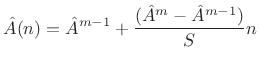
We will not go into the details of solving this equation since McAulay and Quatieri [174] go through every step. We will simply state the result:
| (H.12) |
where
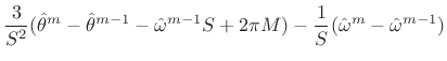 |
(H.13) | ||
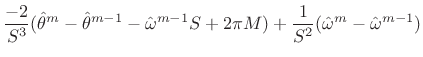 |
(H.14) |
This will give a set of interpolating functions depending on the value of
![$\displaystyle x= {1\over 2\pi} \left[(\hat{\theta}^{m-1} + \hat{\omega}^{m-1} S - \hat{\theta}^m) + (\hat{\omega}^m - \hat{\omega}^{m+1}) {S\over 2}\right]$](http://www.dsprelated.com/josimages_new/sasp2/img3096.png) |
(H.15) |
and finally, the synthesis equation turns into
![$\displaystyle s^m(n) = \sum_{r=1}^{R^m} \hat{A}_{r}^m(n) \cos [\hat{\theta}_{r}^m(n)]$](http://www.dsprelated.com/josimages_new/sasp2/img3097.png) |
(H.16) |
which smoothly goes from frame to frame and where each sinusoid accounts for both the rapid phase changes (frequency) and the slowly varying phase changes.
Figure H.5 shows the result of the analysis/synthesis process using phase information and applied to a piano tone.
![\includegraphics[width=\twidth]{eps/fig8}](http://www.dsprelated.com/josimages_new/sasp2/img3098.png) |
Next Section:
Magnitude-only Analysis/Synthesis
Previous Section:
Parameter Modifications (Step 6)


