Time Scale Modification

Free Books Spectral Audio Signal Processing

Time Scale Modification (TSM) means speeding up or slowing down a sound without affecting the frequency content, such as the perceived pitch of any tonal components. For example, TSM of speech should sound like the speaker is talking at a slower or faster pace, without distortion of the spoken vowels. Similarly, TSM of music should change timing but not tuning.

When a recorded speech signal is simply played faster, such as by lowering its sampling-rate and playing it at the original sampling-rate, the pace of the speech increases as desired, but so does the fundamental frequency (pitch contour). Moreover, the apparent ``head size'' of the speaker shrinks (the so-called ``munchkinization'' effect). This happens because, as illustrated in §10.3, speech spectra have formants (resonant peaks) which should not be moved when the speech rate is varied. The average formant spacing in frequency is a measure of the length of the vocal tract; hence, when speech is simply played faster, the average formant spacing decreases, corresponding to a smaller head size. This illusion of size modulation can be a useful effect in itself, such as for scaling the apparent size of virtual musical instruments using commuted synthesis [47,266]. However, we also need to be able to adjust time scales without this overall scaling effect.

The Fourier dual of time-scale modification is frequency scaling. In this case, we wish to scale the spectral content of a signal up or down without altering the timing of sonic events in the time domain. This effect is used, for example, to retune ``bad notes'' in a recording studio. Frequency scaling can be implemented as TSM preceded or followed by sampling-rate conversion, or it can be implemented directly in a sequence of STFT frames like TSM.

TSM and S+N+T

Time Scale Modification (TSM), and/or frequency scaling, are relatively easy to implement in a sines+noise+transient (S+N+T) model (§10.4.4). Figure 10.17 illustrates schematically how it works. For TSM, the envelopes of the sinusoidal and noise models are simply stretched or squeezed versus time as desired, while the time-intervals containing transients are only translated forward or backward in time--not time-scaled. As a result, transients are not ``smeared out'' when time-expanding, or otherwise distorted by TSM. If a ``transientness'' measure ${\cal T}$ is defined, it can be used to control how ``rubbery'' a given time-segment is; that is, for ${\cal T}=1$ , the interval is rigid and can only translate in time, while for ${\cal T}=0$ it is allowed stretch and squeeze along with the adjacent S+N model. In between 0 and 1, the time-interval scales less than the S+N model. See [149] for more details regarding TSM in an S+N+T framework.

**Figure 10.17:** Time Scaling for S+N+T Models (from [149]).
$\includegraphics[width=0.9\twidth]{eps/scottl-time-scale}$

TSM by Resampling STFTs Across Time

In view of Chapter 8, a natural implementation of TSM based on the STFT is as follows:

Perform a short-time Fourier transform (STFT) using hop size . Denote the STFT at frame and bin by $X_m(\omega_k)$ , and denote the result of TSM processing by $Y_m(\omega_k)$ .
To perform TSM by the factor $\alpha>1$ , advance the ``frame pointer'' by $R/\alpha$ during resynthesis instead of the usual samples.

For example, if $\alpha=2$ ( $2\times$ slow-down), the first STFT frame $X_0(\omega_k)$ is processed normally, so that . However, the second output frame $Y_{1/2}$ corresponds to a time , half way between the first two frames. This output frame may be created by interpolating (across time) the STFT magnitude magnitude spectra of the first. For example, using simple linear interpolation gives

$\displaystyle Y_{1/2}(\omega_k) \eqsp \frac{\left\vert X_0(\omega_k)\right\vert + \left\vert X_1(\omega_k)\right\vert}{2} \,e^{j\theta(\omega_k)}$

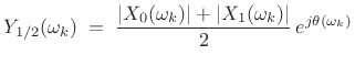(11.23)

where the phase $\theta(\omega_k)$ is chosen to preserve continuity and/or the amplitude envelope from frame to frame under the overlap-add (more on this below). Generalizing to arbitrary TSM factors $\alpha$ , we obtain

$\displaystyle Y_{m}(\omega_k) \eqsp \left[ (1-\eta)\, \vert X_{\left\lfloor m\right\rfloor }(\omega_k)\vert + \eta\,\vert X_{\left\lceil m\right\rceil }(\omega_k)\vert \right]\, e^{j\theta_m(\omega_k)}$

(11.24)

where $\eta\isdeftext m-\lfloor m\rfloor$ , and is advanced by $R/\alpha$ each frame-step.

In general, TSM methods based on STFT modification are classified as ``vocoder'' type methods (§G.5). Thus, the TSM implementation outlined above may be termed a weighted overlap-add (WOLA) phase-vocoder method.

Phase Continuation

When interpolating the STFT across time for TSM, it is straightforward to interpolate spectral magnitude, as we saw above. Interpolating spectral phase, on the other hand, is tricky, because there's no exact way to do it [220]. There are two conflicting desiderata when deciding how to continue phase from one frame to the next:

(1): Sinusoids should ``pick up where they left off'' in the previous frame.
(2): The relative phase from bin to bin should be preserved in each FFT.

To satisfy condition (1), it is necessary to replace the original phase of each frame by the phase corresponding to smooth continuation across time from the previous frame (which is generally an interpolated frame) for each FFT bin. Altering the phase of a spectral frame changes its amplitude envelope in the time domain. Thus, it may no longer looks like a windowed signal segment. Using the WOLA framework (§8.6) helps because the post-window guarantees a smooth cross-fade from frame to frame. Random amplitude-modulation distortion is generally heard as reverberation, also called phasiness [140].

When condition (2) is violated, the signal frame suffers dispersion in the time domain. For steady-state signals (filtered noise and/or steady tones), temporal dispersion should not be audible, while frames containing distinct pulses will generally become more ``smeared out'' in time.

It is not possible in general to satisfy both conditions (1) and (2) simultaneously, but either can be satisfied at the expense of the other. Generally speaking, ``transient frames'' should emphasize condition (2), allowing the WOLA overlap-add cross-fade to take care of the phase discontinuity at the frame boundaries. For stationary segments, phase continuation, preserving condition (1), is more valuable.

It is often sufficient to preserve relative phase across FFT bins (i.e., satisfy condition (2)) only along spectral peaks and their immediate vicinity [142,143,141,138,215,238].

TSM Examples

To illustrate some fundamental points, let's look at some TSM waveforms for a test signal consisting of two constant-amplitude sinusoids near 400 Hz having frequencies separated by 10 Hz (to create an amplitude envelope having 10 beats/sec). We will perform a $2\times$ time expansion ( $2\times$ ``slow-down'') using the following three algorithms:

phase-continued vocoder [70]
relative-phase-preserved vocoder [241,238,143,215]
SOLA-FS [70,104]^11.13

The vocoder STFT frame size is set to 45 ms, the analysis hop size is 1/4 frame, or 11.25 ms, so the analysis frame rate is 89 Hz.

The results are shown in Figures 10.18 through 10.23.

Phase-Continued STFT TSM

Figure 10.18 shows the phase-continued-frames case in which relative phase is not preserved across FFT bins. As a result, the amplitude envelope is not preserved in the time domain within each frame. Figure 10.19 shows the spectrum of the same case, revealing significant distortion products at multiples of the frame rate due to the intra-frame amplitude-envelope distortion, which then ungracefully transitions to the next frame. Note that modulation sidebands corresponding to multiples of the frame rate are common in nonlinearly processed STFTs.

**Figure 10.18:** Phase-continued vocoder waveforms at 2X expansion.
$\includegraphics[width=\twidth]{eps/pv-ellis-wave}$

**Figure 10.19:** Phase-continued vocoder spectra at 2X expansion.
$\includegraphics[width=\twidth]{eps/pv-ellis-spec}$

Relative-Phase-Preserving STFT TSM

Figure 10.20 shows the relative-phase-preserving (sometimes called ``phase-locked'') vocoder case in which relative phase is preserved across FFT bins. As a result, the amplitude envelope is preserved very well in each frame, and segues from one frame to the next look much better on the envelope level, but now the individual FFT bin frequencies are phase-modulated from frame to frame. Both plots show the same number of beats per second while the overall duration is doubled in the second plot, as desired. Figure 10.21 shows the corresponding spectrum; instead of distortion-modulation on the scale of the frame rate, the spectral distortion looks more broadband--consistent with phase-discontinuities across the entire spectrum from one frame to the next.

**Figure 10.20:** Phase-locked vocoder waveforms at 2X time expansion.
$\includegraphics[width=\twidth]{eps/pv-salsman-wave}$

**Figure 10.21:** Phase-Locked Vocoder Spectra at 2X Time Expansion.
$\includegraphics[width=\twidth]{eps/pv-salsman-spec}$

SOLA-FS TSM

Finally, Figures 10.22 and 10.23 show the time and frequency domain plots for the SOLA-FS algorithm (a time-domain method). SOLA-type algorithms perform slow-down by repeating frames locally. (In this case, each frame could be repeated once to accomplish the $2\times$ slow-down.) They maximize cross-correlation at the ``loop-back'' points in order to minimize discontinuity distortion, but such distortion is always there, though typically attenuated by a cross-fade on the loop-back. We can see twice as many ``carrier cycles'' under each beat, meaning that the beat frequency (amplitude envelope) was not preserved, but neither was it severely distorted in this case. SOLA algorithms tend to work well on speech, but can ``stutter'' when attack transients happen to be repeated. SOLA algorithms should be adjusted to avoid repeating a transient frame; similarly, they should avoid discarding a transient frame when speeding up.

**Figure 10.22:** SOLA-FS waveforms at 2X expansion.
$\includegraphics[width=\twidth]{eps/pv-solafs-wave}$

**Figure 10.23:** SOLA-FS spectra at 2X expansion.
$\includegraphics[width=\twidth]{eps/pv-solafs-spec}$