


Welch's Method
Welch's method [296] (also called the periodogram method) for estimating power spectra is carried out by dividing the time signal into successive blocks, forming the periodogram for each block, and averaging.
Denote the ![]() th windowed, zero-padded frame from the signal
th windowed, zero-padded frame from the signal ![]() by
by
 |
(7.26) |
where
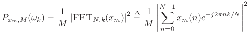
as before, and the Welch estimate of the power spectral density is given by
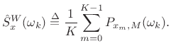
In other words, it's just an average of periodograms across time. When
Welch Autocorrelation Estimate
Since
![]() which is circular (or
cyclic) correlation, we must use zero padding in each FFT in
order to be able to compute the acyclic autocorrelation function as
the inverse DFT of the Welch PSD estimate. There is no need to
arrange the zero padding in zero-phase form, since all phase
information is discarded when the magnitude squared operation is
performed in the frequency domain.
which is circular (or
cyclic) correlation, we must use zero padding in each FFT in
order to be able to compute the acyclic autocorrelation function as
the inverse DFT of the Welch PSD estimate. There is no need to
arrange the zero padding in zero-phase form, since all phase
information is discarded when the magnitude squared operation is
performed in the frequency domain.
The Welch autocorrelation estimate is biased. That is, as
discussed in §6.6, it converges as
![]() to the true
autocorrelation
to the true
autocorrelation ![]() weighted by
weighted by ![]() (a Bartlett window). The
bias can be removed by simply dividing it out, as in
(6.15).
(a Bartlett window). The
bias can be removed by simply dividing it out, as in
(6.15).
Resolution versus Stability
A fundamental trade-off exists in Welch's method between
spectral resolution and statistical stability.
As discussed in §5.4.1, we wish to maximize the block size
![]() in order to maximize spectral resolution. On the other
hand, more blocks (larger
in order to maximize spectral resolution. On the other
hand, more blocks (larger ![]() ) gives more averaging and hence
greater spectral stability.
A typical default choice is
) gives more averaging and hence
greater spectral stability.
A typical default choice is
![]() , where
, where ![]() denotes the number of available data
samples.
denotes the number of available data
samples.
Next Section:
Welch's Method with Windows
Previous Section:
The Periodogram


