


An Interesting Fourier Transform - 1/f Noise
Power law functions are common in science and engineering. A surprising property is that the Fourier transform of a power law is also a power law. But this is only the start- there are many interesting features that soon become apparent. This may even be the key to solving an 80-year mystery in physics.
It starts with the following Fourier transform:

The general form is tα ↔ ω-(α+1), where α is a constant. For example, t2 ↔ ω–3 and t -0.75 ↔ ω–0.25. Unfortunately, there are additional terms that distort this simple relation. First, the left side contains the term, u(t), the unit step function. This is defined as u(t) = 0 for t < 0, and u(t) = 1 for t ≥ 0. In other words, this makes the time domain a one-sided power law. Second, the power law in the frequency domain only pertains to the magnitude; there is a phase term that doesn't resemble a power law at all. Third, there is a scaling factor in the frequency domain, Γ(α +1). This is the Gamma function, which is essentially a continuous version of factorials. A graph of the Gamma function is shown below. Don't worry too much about this strange function. Think of it simply as a constant that scales the amplitude of the frequency domain, depending on the value of α.

The table below shows nine cases of this Fourier transform, with alpha running from -2.0 to 2.0, and rough sketches of the curves. The frequency domain also shows a rough sketch of the magnitude graphed on a log-log plot, which turns out to be is a straight line with a slope of -(α+1). Take a few minutes to examine this figure, especially noting the symmetry between the time and frequency domains.

One of these cases should be familiar to you, where α=0. This is the Fourier transform of the unit step function, with a magnitude of 1/ω, and a phase of -π/2. As you probably recall, this describes the impulse and frequency response of the perfect integrator. Now consider the case of an integrator followed by another integrator. The impulse response of this two stage combination is the unit step response convolved with itself. In the frequency domain the magnitude becomes 1/ω × 1/ω, and the phase becomes 2 × (-π/2). This two-integrator cascade is shown on the graph for α=1, where the impulse response is a linearly increasing line, and the frequency spectrum is 1/ω2 , with φ = -π. Likewise, α=2 represents a cascade of three integrators, and so on. It is interesting that these Fourier transforms are so well behaved, in spite of both domains containing nasty features (such as: t2 as t → ∞ , and ω-3 as ω → 0 ).
Here is something even more interesting. As you approach α = -1, the time domain approaches a shape of t-1, and the frequency domain approaches a flat magnitude with a zero phase. However, a flat magnitude and zero phase corresponds to a delta function, δ(t), in the time domain. That is, in the limit as α → -1, u(t)t-α = δ(t). This is because the sharp point of t-α grows rapidly as α → -1, dominating the entire function. But what happens exactly at α = -1? How could the sharp point ever completely negate the seemingly finite width of t-1? The mathematics tells you not to ask this question. Recall that the frequency domain has a scaling factor of Γ(α+1). For α = -1, the gamma function is undefined.
Now we come to a feature that I find absolutely fascinating. In general, we have seen that a power law in one domain corresponds to a power law in the other domain. Further, there is an inverse relationship; if the time domain decays faster, then the frequency domain decays slower, and vice-versa. This means that there must be a certain decay rate that is unique, where both domains are equal. This occurs for α = -0.5, where the time domain is t-0.5 and the frequency domain is ω-0.5. Interesting, but what does this mean?
Now look at the figure below, a graph of the measured noise that originates within a common electronic amplifier. The flat section above 100 Hz is called white noise , and is well understood. However, the sloping portion below 100 Hz is not well understood at all. This is 1/f noise, a mystery that has resisted explanation for over 80 years. 1/f noise has been observed in the strangest places- electronics, traffic density on freeways, the loudness of classical music, DNA coding, and many others.

Many of the properties of noise are directly related to the amount of power in a signal, that is, to the square of the amplitude. Accordingly, most of those working with noise think in terms of power spectra, not amplitude spectra. 1/f noise gets its name because its power spectrum has a shape that is close to 1/f. However, if we look at the amplitude spectrum for 1/f noise it has a shape of 1/f1/2. As can be seen above, on a log-log plot of amplitude, 1/f noise has a slope of -0.5. Now you can see where I’m going.
At least in a limited sense, 1/f noise is its own Fourier transform, with ω-1/2 in the frequency domain, and t-1/2 in the time domain. For instance, a single pulse given by u(t) t-1/2 has a 1/f power spectrum. Likewise, a randomly occurring sequence of such pulses has a 1/f power spectrum, at least over a wide range frequencies. Further, 1/f noise can be created by passing white noise through a filter with an impulse response of u(t) t-1/2. Unfortunately, none of these scenarios seems to have a physical interpretation that explains the widespread observation of 1/f noise. It’s clear that something is still missing.
There is also another issue: u(t) t-1/2 is the transform pair of Mag = ω-1/2 , φ = -π/4. However, no one knows what the phase of 1/f noise is, or even if it has a defined phase. If the phase happens to be different from φ = -π/4, then the corresponding time domain signal will also be different. That is, it may be that the characteristic time domain waveform of 1/f noise is simply not t-1/2.
Nevertheless, the idea that 1/f noise is its own Fourier transform is very compelling. Consider the Gaussian curve, the most important waveform associated with random events. The Central Limit Theorem tells us why the Gaussian is so commonly observed. However, it is also true that the Fourier transform of a Gaussian is a Gaussian. This seems more than coincidence– I think it is a critical clue in solving the mystery of 1/f noise.
Comments are certainly welcome! I especially appreciate suggestions for new directions in research and (god forbid) errors in math.
Steve Smith email http://www.dspguide.com/
11/24/2007


- Comments
- Write a Comment Select to add a comment
Does anyone have a reference for the result that the FT of a power law is a power law? I have been hunting for one and can't find it. Thanks
Hi Steve,
I've also pondered the origin of 1/f noise as a hobby over the years. The 2004 paper "Thermal-Noise Limit in the Frequency Stabilization of Lasers with Rigid Cavities," was a small breakthrough. It explained the 1/f frequency noise in a stabilized laser as being due to Brownian motion "thermal noise" in the bits that make up the frequency reference. The frequency reference is an ultra-stable ceramic spacer with high-quality mirrors at either end, making a Fabry-Perot cavity. And the tiny observed 1/f noise, 1 part in 10^15 fractional of spacer length and consequently of the laser optical frequency, is explained as originating in thermal noise that alters the length of the spacer and the thickness of the mirror coatings. Kenji Numata was the first to notice that this explanation worked over a large range of Fourier frequencies and mechanical constructions techniques.
The natural question is are there other examples of 1/f noise that can be explained by thermal noise? So far, I've come up with one candidate. This 2016 paper , "Study on the origin of 1/f noise in quart resonators" concluded the origin of 1/f noise is unexplained. But Equation (8) and the measurements hint strongly at thermal noise being the origin, the same as for the laser frequency reference.
Love your DSP book!
Bob
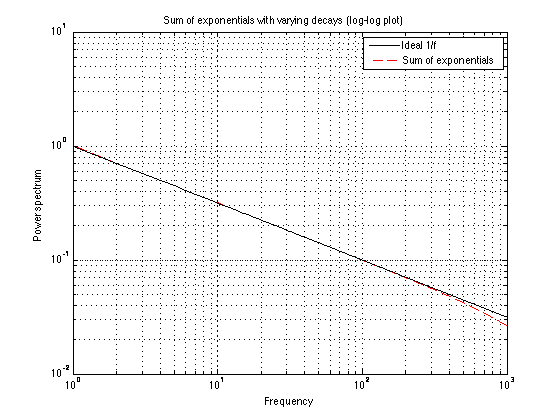
A natural model of flicker noise (1/f) arrives from adding a few or more independent exponential decays if the time constants of each are "greatly varied". It would seem surprising that you can get 1/f by adding together many 1.0 / (a_k^2 - f^2) -- but a quick simulation shows it to be true.
f = 1:1000; y_pow = zeros(size(f));
for a=1:1000
    f_x =  1.0 ./ (a + 1i*f); % Fourier transform of exp(-a*t)
    y_pow = y_pow + f_x.^2; % power adds for independent signals
end

loglog(abs(sqrt(y_pow)), 'r'); hold on;
loglog( 1./sqrt(f) , 'k');
Based on reference: Bell D.A. (1960) Electrical Noise Fundamentals & Physical Mechanism
Hi Steve,
13 years after writing "no one knows what the phase of 1/f noise is, or even if it has a defined phase." have you/us gained a better understanding?
I'm still puzzled by that.
Please let me know if you any pointers to new information available.
Thank you!
Best regards,
Alberto
Please see my comment , below.
Hi, I did some thinking on this in the 80's; relating to signal processing at S/N close to 1 :)
If anybody is interested I have a brief write-up at: https://en.wikipedia.org/wiki/User:Rrogers314
I posted on Wikipedia but some "hall monitor" kicked it out, but I kept it on my talk page.
The essence is we don't have a universe big enough for the limit, but we do have systems/detectors that show the 1/f noise slope. The solution is to acknowledge that we always calibrate/auto-zero. Then the 1/f equation gives random "drift" and accumulated drift goes as the Cin() function. In my case I had a detector that had 1/f (really neat on an analyzer). So I put in "auto-calibration/zero"; the circuit performance corresponded to that attitude. I also found it in the 80's audio delta-sigma converters, with a knee at 100hz.
If anybody is interested I can get more detailed. I thought it was a neat derivation:)
Ray

Flicker noise (1/f noise) is white noise in frequency, or the noise due to frequency fluctuations is constant over the range of frequencies considered. This can be confusing since we are referring to frequency in two different aspects when considering the power spectral density due to frequency fluctuation: similar to using frequency deviation and frequency modulation when discussing standard Frequency Modulation. Frequency is the time derivative of phase (a change in phase versus a change in time is instantaneous frequency), so when the same noise process is viewed on a phase power spectral density (the typical phase noise plot and due to small angle approximations the same thing we would see on a spectrum analyzer when phase noise is dominant), it will be 1/f noise since the phase, as the integral of frequency will be going down at 1/f (integration is a low pass filter), resulting in the phase PSD going down at -20 dB/decade when the noise is a white-FM process.

Thanks Steve. This is a wonderful and stimulating article. I like this kind of observations/interpretations. This is what makes math 'beautiful'. The moment I read this, the first thing that strikes my mind is the theory of eigenvalues and vectors. So many problems become much easier when though-off as matrices. When the signal is sampled, FT is replaced with DFT which can simply be denoted by the multiplication of matrix and vector. If F is the DFT matrix and x is a vector, then xf=Fx, and xf is the DFT of x. We are looking at vectors (signals) x that satisfy Fx = \lamda x where \lamda is an eigenvalue of the transformation x. We know from matrix theory that there could be an infinite number of eigenvectors for a matrix A but then no of non-zero eigenvalues cannot exceed the rank of matrix A, and that the space spanned by the eigenvectors is the null space of A and its dimensionality is determined by the rank of A as well. In your other article 'waveforms that are their own fourier transform' , you clearly show that the no of eigenfuncions (functions who shape remains the same under FT) is infinite. The same conclusion can be achieved through linear algebra as well. For DFT, the eigenvectors would span a finite-dimensional space N and for continuous FT, the eigenfunctions would span an infinite dimensional space and so on.
Anyways, coming back to the interpretation of the 1/f noise's PSD being an eigenfunction of FT - since Gaussian function can be expanded into polynomials, it is not very surprising that power law functions satisfy the same property. I think the uniqueness of flicker noise is the following. While the probability distribution itself is an eigenfunction (Gaussian), it time correlation is also an eigenfunction. Dont know if this would help solve the mystery. But enjoyed it.
Hi Steve,
"Unfortunately, none of these scenarios seems to have a physical interpretation that explains the widespread observation of 1/f noise. It’s clear that something is still missing."
Some thoughts about that:
Electrical current is represented by moving electrons in some conductor or semi-conductor. This materials all have a internal cristallin structure. And as an universal rule told us, nothing is perfect, this cristallin structures contains damages effecting the flow of electrons somehow.
Guess we have an artificial watercourse with really smooth edges. Now we put leaves on it, normal distributed, and count the leaves comming along per time unit some where down the stream. We will see, the recorded numbers will follow more or less a normal distribution.
Guess we have a natural watercourse with rough edges (Banks). We do the same experiment. This time some leaves will stuck at a point along the banks. After a while some other leave will stuck at the same position, and we will see a growing collection of leaves stucking at this position. The recorded numbers of leaves is less now. One more leave and the collection break free. In opposite to its 'construction' this collection breaks free and swim down as a collection of leaves. This produces a high peak in our counts of leaves per time unit. (Some times flicker noise is also called Popcorn noise, especially by Audio engineers)
And it needs time for the collection to grow. So, lager collections (peaks) will be observed very seldom relative to smaller collections ==> 1/f.
Unfortunately, electrons carrying a negative charge and so want to maximize her distance, leaves do not. I am not that good in physics or mathematics to overcome that problem, its just an idea.
Sorry for my english, hope you get the big picture ....
With best regards
Gerhard
Dear Steve Smith,
this article helps me a lot in my research. Can you provide some reference (book or, even better, papers) that states the first formulae in the box, it is very important for me. I am struggling in this problem for weeks.
Hi Mardy,
E-mail me at Steve.Smith "at" Tek84.com
and I'll give you some help.
Steve
Thank you Steve. I found the references at the end. Thank you. I am thinking about this article over and over again. I have a question now:
If I well understood, the fact that I have 1/f noise spectrum, can imply a power law behavior of the time history of the signal which is t^(-a). Are there some implications in this? Should pink noise signal, for instance, have a degrowth?
Came by this dated but interesting note.
When asked about the logic behind 1/f noise I like to refer to something easy to relate to.
Take the amplitude of the AC voltage in a power socket - usually its around 230/110V with some smaller and frequent variations.
Occasionally there is a power cut but it happens rarely i.e. it is a low frequency event but the amplitude is big.
And occasionally lightening strikes nearby - it is rare with a direct hit but the amplitude is very big and it happens at low frequencies.
And to the extreme, some day the sun flares up and wreck havoc,, well you get the idea.
To post reply to a comment, click on the 'reply' button attached to each comment. To post a new comment (not a reply to a comment) check out the 'Write a Comment' tab at the top of the comments.
Please login (on the right) if you already have an account on this platform.
Otherwise, please use this form to register (free) an join one of the largest online community for Electrical/Embedded/DSP/FPGA/ML engineers:


