


Understanding Radio Frequency Distortion
Overview
The topic of this article are the effects of radio frequency distortions on a baseband signal, and how to model them at baseband. Typical applications are use as a simulation model or in digital predistortion algorithms.
Introduction
Transmitting and receiving wireless signals usually involves analog radio frequency circuits, such as power amplifiers in a transmitter or low-noise amplifiers in a receiver.
Signal distortion in those circuits deteriorates the link quality. When designing wireless devices, distortion is an important design problem, since the need for more linear components can significantly increase cost and power consumption.
Negative frequencies
A short excourse on negative frequencies:
Radio frequency amplifiers process real-valued signals: The waveform is a voltage or a current, and could be shown for example on an oscilloscope. For real-valued signals, the negative frequencies are always a "mirror image" of the positive frequencies, they hold no additional information. We tend to forget about them, knowing that the signal is real-valued.
However, the negative frequency components allow a rather straightforward explanation of distortion products.
A (co)sine wave can be constructed as a sum of two complex exponentials:
(1) 
If cos(...) describes a carrier wave, then the exp(...+f) and exp(...-f) terms can be interpreted as its positive and negative frequency component, respectively.
Clearly, the two exp(...) terms are complex conjugates of each other, and the same applies to any signal:
For a real-valued signal, positive and negative frequency components are complex conjugate.
Baseband and radio frequency signals
A radio frequency signal is modulated to a carrier wave at a carrier frequency fc. Often, the carrier wave is generated in a radio frontend and used to up- or downconvert signals. However, depending on the transceiver architecture, it can be a purely mathematical construct. For simplicity, assume that fc is located in the middle of the transmit bandwidth, for example 2.462 GHz for 802.11b channel # 11.
Fig. 1 spectrum of a radio frequency (RF) signal
If the bandwidth of the signal is for example 22 MHz, then 99 % of the spectrum are empty.
In digital signal processing, the carrier frequency is omitted, and an equivalent baseband signal is used instead:
Fig. 2 spectrum of the baseband equivalent signal
The baseband-equivalent signal is obtained from the RF signal by
- shifting the positive frequency component to 0 Hz
- discarding the negative frequency component
In other words:
The baseband-equivalent signal is the positive frequency component of the RF signal, shifted to 0 Hz.
Since its positive and negative frequency components are independent, the baseband-equivalent signal is complex-valued.
Converting a baseband-equivalent signal to RF
The RF signal can be reconstructed from the complex baseband-equivalent signal BB(t) by:
- shifting BB(t) to fc
- shifting BB*(t) to -fc: This reconstructs the negative frequency component, the asterisk denotes complex conjugation.
In equations, this can be written as follows (based on eq. 1.11 in [1], scaling factors are omitted for brevity).
(2) RF(t)=BB(t)exp(2i pi fc t)+BB*(t)exp(-2i pi fc t)
All exp(...) terms can be interpreted as rotating phasors with a given frequency. They are rewritten using a "carrier wave function":
(3) carrier(f, t)=exp(2i pi f t)
Eq. (2) now becomes
(4) RF(t)=
(4.1) BB(t)carrier(fc, t)
(4,2) +BB*(t)carrier(-fc, t)
Comparing with the spectrum in Fig. 1, the two terms correspond to positive and negative frequency components, respectively.
Distortion in RF components
Distortion results, when the input-output relation of analog components, such as transistors, is nonlinear. For example, the maximum output voltage of an amplifier is limited by the available supply voltage. Any attempt to drive it to a higher level will result in clipping of the waveform, causing severe distortion.
When a transceiver is properly designed and operated within its specifications, such extreme distortion should happen only rarely. To make the problem mathematically tractable, it is often assumed that circuits are operated in the weakly nonlinear regime. For a weak nonlinearity, the input-output relationship can be approximated using a polynomial of the input signal:
(5) RFout(t) = a0 + a1 RFin(t) + a2 RFin(t)2+...a3 RFin(t)3+...
Most frequently, 3rd order polynomials are used. Sometimes the analysis is extended to 5th and 7th order. For higher orders, the accuracy improves only marginally, since polynomials extend asymptotically to infinity, whereas a "strong" nonlinearity always approaches a finite limit, such as the supply voltage of the circuit.
The coefficients [a0, a1, a2, a3, ...], together with eq. (4), form a model for the amplifier. However, the model in its current form is not too convenient for DSP engineering, since it relies on the radio-frequency waveform instead of the baseband-equivalent signal.
The signal RF(t) from (4) is inserted for RFin(t) in (5), and the resulting products are examined. For a baseband-equivalent model, we are only interested in distortion products that re-appear at the carrier frequency fc. Other terms (for example harmonics at multiples of fc) will be omitted.
First, there is coefficient a0. It appears as a constant term at 0 Hz and can be discarded since it does not appear at the carrier frequency.
Next, a1 passes the input signal to the output. It corresponds to the gain of the amplifier. For a weakly nonlinear system, a1 RFin(t) is always the dominant term. It is included in a baseband-equivalent model, since the signal appears at the original carrier frequency.
With coefficient a2, things start to get interesting: RFin(t) is squared.
2nd order distortion product
The second-order distortion term in (5) is a2 RFin(t)2.
Further, according to (4), RFin(t) is the sum of a positive frequency term, let's call it 'a' and a negative frequency term 'b'.
Simple multiplication results in (a+b)2=a2+2ab+b2.
The square of the positive frequency term a is BB(t)2carrier(fc, t)2.
Looking at eq. (3), the square of a carrier wave is a carrier at twice the frequency: carrier(fc, t)2=carrier(2 fc, t)
More generally, any product of carriers results in a carrier at the sum frequency (note that carrier waves are complex-valued, and no difference frequency products are created, as would be the case with sine waves):
(6) carrier(f1, t) carrier(f2, t) = exp(2i pi f1 t) exp(2i pi f2 t) = exp(2i pi (f1+f2) t) = carrier(f1+f2, t)
Writing out the products,
(7) RFin(t)2=
(7.1) + BB(t)2carrier(2 fc, t)
(7.2) + BB(t) BB(t)*
(7.3) BB*(t)2 carrier(-2 fc, t) .
The terms can be interpreted as
- (7.1): BB(t)2 at twice the carrier frequency
- (7.2): the product of BB(t) and its conjugate at 0 Hz
- (7.3): the negative-frequency mirror-image of (7.1)
To convert (7) into a baseband-equivalent signal, we drop all terms that do not include carrier(fc, t) (remember, a baseband equivalent signal is the positive frequency component around a RF carrier, other parts are omitted).
Surprisingly, nothing remains! As long as the assumptions hold (narrowband signal, weakly nonlinear), a second-order nonlinearity does not contribute any distortion to the band around the carrier frequency.
However, second-order distortion can become a problem in mixer circuits, when the (7.2) component at DC appears inside a mixer circuit and bypasses the mixer's frequency conversion as a result of circuit imbalance.
In radio receivers, a strong narrow-band interferer can up-convert term (7.2) close to the carrier frequency. This process is known as cross-modulation. While the distortion product is identical to (7.2), shifted to the interferer's frequency, crossmodulation is strictly speaking a third-order nonlinear process.
3rd order distortion product
For distortion in any practical circuit, a3 is by far the most important contributor.
The calculation is easily carried out starting from eq. (7), using RFin(t)3= RFin(t)2 RFin(t). For a complex baseband-equivalent of the distortion product, we are only interested in products that appear around fc. Only the product of (7.1) with (4.2) falls to the frequency range of interest:
(8) carrier(2 fc, t) BB(t)2 carrier(-fc, t) BB*(t)
= carrier(fc, t) |BB(t)|2 BB(t)
Higher order distortion product
The discussion of the 2nd and 3rd order distortion product can be generalized as follows:
The complex-baseband equivalent of the distortion product is zero for all even orders. The reason is that the distortion product does not fall into the frequency band around the carrier, if the narrow-band assumption holds.
For odd orders, the complex-baseband equivalent of the distortion product can be calculated as
(9) distn(t)= |BB(t)|(n-1) BB(t)
Note that after dropping the carrier(fc, t)-factor, all distortion products are independent of the carrier frequency. For the model, it does not matter, whether we operate at 2 GHz or at 60 GHz (of course, real circuits are frequency dependent).
Practical example
As a practical example, here are the coefficients of one particular power amplifier I have characterized in the lab (more information in [2], [3]):
a1 1.02275 − 0.10838i
a3 0.16800 + 0.17700i
a5 −0.16218 − 0.09233i
a7 0.04108 + 0.02196i
a9 −0.00434 − 0.00239i
a11 0.00016 + 0.00009i
Using those coefficients together with (9) and a baseband signal with unity RMS amplitude models the amplifier quite accurately, as long as the instantaneous magnitude of the input signal doesn't exceed the range used during measurement.
Bandwidth of distortion products
When implementing eq. (9) in Matlab etc, it is important to note that the bandwidth of the n-th order distortion product is n times the bandwidth of the input signal. The reason is that each multiplication of BB(t) with itself (or a conjugate) results in a convolution of the spectra.
Fig. 3 Spectrum of higher-order distortion products in complex baseband-equivalent signal
Ideally, the oversampling factor should be at least the order of the model. This prevents any alias products folding back into the frequency range of the wanted signal.
It is important to note that the spectrum of an n-th order nonlinearity is exactly confined to n times the original bandwidth. This can make lower-order models more convenient in simulations, since unwanted alias products can be prevented to cause aliasing. However, it also shows that for example a 3rd-order model is clearly insufficient to predict unwanted emissions into "alternate" channels (see Fig. 3).
Matlab example
To illustrate the ideas, here is a short Matlab example: download
It generates an OFDM stream, creates several distortion products, and combines 3rd / 5th order products into a simple power amplifier model ("ballpark numbers" for a cellular wireless transmitter, but not based on any real-world component. Maybe it's a bit too nonlinear, but the idea here is to show the distortion products).
The simulation uses a cyclic signal stream, similar to an arbitrary waveform generator in the lab that periodically repeats the same sequence. This allows ideal, non-causal "brickwall" filtering and shows clearly the bandwidth of the distortion products for an ideally bandlimited signal.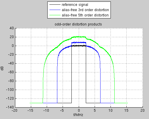
Fig. 4 Input signal, 3rd and 5th order distortion products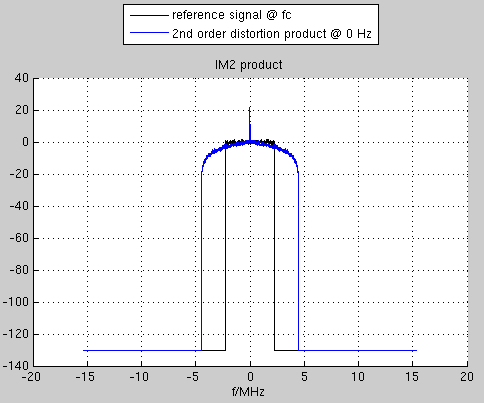
Fig. 5 Input signal and 2nd order distortion product (note: usually it does not appear at the same frequency)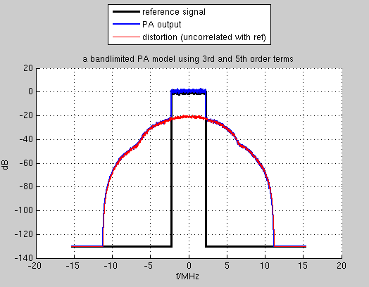
Fig. 6 A simple PA model. The inband distortion is uncorrelated with the signal and would appear to a receiver as error vector magnitude
Summary
- A complex baseband equivalent signal is the positive frequency component of a radio frequency signal at a carrier frequency, shifted to 0 Hz.
- Distortion products in a nonlinear amplifier are created as products between positive and negative frequency component
- Only a few distortion terms appear at the carrier frequency, making them eligible for use in a baseband-equivalent model. Those terms are invariant with carrier frequency.
- Those distortion terms have odd order and can be computed from the baseband-equivalent signal as |BB(t)|(n-1) BB(t).
- The bandwidth of the n-th order distortion product cannot exceed n times the bandwidth of the input signal.
References
[1]: Complex Baseband Representation of Bandpass Signals
[2]: Optimizing spectral shape under general spectrum emission mask constraints
[3]: Power amplifier characterization for predistortion in mobile transmitters


- Comments
- Write a Comment Select to add a comment
Great article.
BTW. In (5) the a0, a1, a2 are by definition real (since RF_in(t)/RF_out(t) are real). Can You explain
why they turn out complex in the practical example? Does it follow from dynamic nonlinearities ?
Regards,
Alek.

good point.
This is simply missing from Eq. 5.
Its purpose was to illustrate, how a nonlinearity at RF becomes a complex-baseband equivalent model. But, it's not a complete formal derivation:
Eq. (5) doesn't account for memory effects (AMPM) but the example PA _does_ suffer from AMPM distortion.
To fit this together, we'd need additional terms for the imaginary part of the coefficients in Eq. (5).
They need to include some Hilbert-transform-like structure acting on the RF signal, to turn sine into cosine, and vice versa.
To post reply to a comment, click on the 'reply' button attached to each comment. To post a new comment (not a reply to a comment) check out the 'Write a Comment' tab at the top of the comments.
Please login (on the right) if you already have an account on this platform.
Otherwise, please use this form to register (free) an join one of the largest online community for Electrical/Embedded/DSP/FPGA/ML engineers:


