


Understanding and Relating Eb/No, SNR, and other Power Efficiency Metrics
Introduction
Evaluating the performance of communication systems, and wireless systems in particular, usually involves quantifying some performance metric as a function of Signal-to-Noise-Ratio (SNR) or some similar measurement. Many systems require performance evaluation in multipath channels, some in Doppler conditions and other impairments related to mobility. Some have interference metrics to measure against, but nearly all include noise power as an impairment. Not all systems are mobile or required to work in multipath channels or in the presence of interferers or other impairments, but nearly all communication systems include Low Noise Amplifiers in their receivers and when the input signal is weak the thermal noise in the amplifiers in the Analog Front End (AFE) of the receiver starts to dominate the performance impairments of the system. Understanding and properly calculating the various metrics related to SNR and power efficiency is important for analysis purposes but often a stumbling block and minefield of potential errors. This article attempts to clarify some of the basic metrics and their use.
Understanding and Estimating SNR
The most basic metric is the Signal-to-Noise-Ratio (SNR), which is simply the ratio of the received signal power, Ps, to the in-band noise power, Pn. The in-band noise power is typically fairly constant, sometimes slowly varying with the temperature of the receiver. The amplitude distribution of thermal noise is Gaussian and it’s nature is additive with respect to the signal, so it is generally referred to (and modeled as) Additive White Gaussian Noise (AWGN). This noise is generated within the receiving elements of the analog components of the receiver, and the majority usually comes from the Low Noise Amplifier (LNA). The LNA is so-called because it is designed to generate the lowest noise possible because it is known that the noise from the LNA will be a strong contributor, if not the strongest contributor, to the total receiver noise power, since any subsequent amplification stages will amplify the noise from the LNA along with the signal. Well-designed receivers have thermal noise that is spectrally flat, and the power will be proportional to the receiver “noise temperature”, T, in Kelvin, and bandwidth, B, in Hertz, as related by Boltzmann’s constant in Johnson’s equation [1] as shown in Eq. 1.
Pn = kTB (1)
The subscript ‘n’ indicates that the power, Pn, is contributed only by the noise, which is generally taken to be the thermal noise described by Eq. 1.
The signal power is, intuitively, the total power incident at the receiver contributed only by the desired signal. Letting the desired signal power level be indicated by Ps, the SNR is then simply:
SNR = Ps/Pn (2)
Generally SNR is expressed in deciBels (dB). Note that the received SNR may be different at different points in the receiver, as various components, such as amplifiers, mixers, filters, etc., all add small amounts of noise to the total noise power. The sum of the noise contributions of the various components in the receive chain is often called the “Noise Figure” (NF) of the receiver. Likewise digital processing can add noise in the form of quantization errors and other effects, and while these noise sources contribute to the total noise that may be seen at a detector or slicer, they are not the same as the thermal noise and may have different statistical distributions.
Communication signals are always bandlimited due to practical and regulatory considerations, so methods for measuring the signal power, Ps, are generally straightforward. The noise, however, has infinite bandwidth in the ideal model and practically always greater, and usually much greater, bandwidth than the signal in the receiver front end. For a well-designed receiver and demodulator the noise within the region of the signal bandwidth will determine the effective SNR. This does, however, raise the question of how one should properly measure Pn, the noise power, in order to estimate the SNR. The basic definition of Pn in Eq. 1 includes bandwidth, B, in the computation, but unless the practical noise has a brick wall-shaped spectrum with width B then Eq. 1 will not precisely describe the noise power in practice. There are a number of ways, however, to measure SNR but they may differ depending on the context, what the measurement will be used for, and other considerations. This often results in practical disagreements regarding the definition of SNR, and what it generally boils down to is that there are some contextual dependencies on the definition. Some example considerations may include whether multipath reflections, pilot tones or training sequences are included in the received signal power, what the measurement bandwidth of the noise (and sometimes signal) power should be, and at what point along the receiver or demodulator signal chain the SNR should be measured.
Using SNR as a performance metric has some limitations that are important to understand. Since the noise power definition in Eq. 1 and it’s practical measurement depend on the bandwidth of the noise, if the signal changes bandwidth, even if the signal power is held constant, the noise measurement bandwidth may need to change as well. Reducing the noise bandwidth will decrease the noise power resulting in an increase in SNR even though there was no increase in signal power. The increase in SNR due to decreased signal bandwidth is often referred to as “power concentration” and can yield an increase in range or reliability at the expense of data rate. From a system analysis perspective it means that SNR must be interpreted carefully when comparing systems or configurations. Comparing systems or configurations that use the same signal bandwidth and definition of SNR is practical, but comparing systems with differing signal bandwidths or SNR definitions requires careful attention to details and consideration of such things as the effects of power concentration.
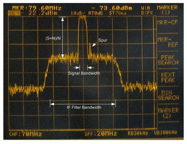
A related blog article, Some Observations on Comparing Efficiency in Communication Systems, also discusses power concentration with an illustration in Figure 9 of that article. As mentioned there, another way to look at SNR is as a comparison of the Power Spectral Densities (psd) of the signal and the noise. Since psd is expressed with units of power per unit bandwidth, this removes the bandwidth uncertainty for the noise power measurement. It does not, however, address the problem of being able to compare signals of different bandwidth, since changing the bandwidth of a signal with constant power changes its psd. One advantage of using psd values rather than total integrated power is that it can be measured with reasonable accuracy using a Spectrum Analyzer. Figure 1 shows a Spectrum Analyzer display with a single-carrier 64QAM signal in noise after IF filtering. The shape and bandwidth of the IF filter can be easily seen and the signal energy psd is aligned with the top of the display area. The noise level of interest is not that outside of the IF filter passband, which is likely the noise floor of the Spectrum Analyzer, but the noise level in the IF filter passband near the desired signal energy. The difference in psd of the signal and noise will be the ratio (S+N)/N as shown in Fig. 1. The display shows that the analyzer is set at 10dB/div and three divisions of the display graticule are covered so that (S+N)/N = 30dB. The SNR can be calculated by converting to linear, subtracting one (1), and then back to dB as follows:
SNRlin = 10SNN/10 -1 = 999 Eq. 1, Converting (S+N)/N to linear SNR
SNRdB = 10log(SNRlin) = 29.9957 dB
where SNN is the observed (S+N)/N ratio. In this case there is barely any difference between SNR and (S+N)/N, but at lower SNRs the difference can be more significant.
Estimating SNR with a Spectrum Analyzer is only as good as the precision of the estimation of the psd of the signal and noise levels, which is done visually and subject to error. It is, however, generally good for a workable SNR estimate and can easily reject spurious or other adjacent energy that might otherwise get measured as either signal or noise power. A significant spur can be seen just to the right of the signal energy in Fig. 1. The energy in that spur would likely affect instrumented or numeric estimates of the SNR, but can be easily rejected by inspection of the display when estimating (S+N)/N.
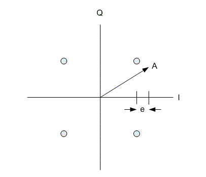
It is also possible to make an estimate of SNR in the demodulator during symbol detection or slicing. Figure 2 shows an example of a particular received symbol, A, and it’s error component, e, in the I channel. An independent error component will also exist in the Q channel, but since the noise power is statistically equal in both the I and Q channels it does not need to be computed in both. Estimating the in-band noise power from the sequence of sliced error components in either the I or Q channel will generally be accurate as long as AWGN dominates the signal impairments at the slicers. If there is Intersymbol Interference (ISI), synchronization errors, receiver distortion or other significant impairments the effects of these will be included in the sliced error component. The magnitude of the desired sliced symbol provides the signal energy component in the I channel.
Bandwidth Independent Metrics
In order to compare systems independent of either the signal or noise bandwidth, it is necessary to use metrics for both signal level and noise level that are bandwidth independent. For the noise level it is convenient to use psd in the form of No, which is the noise power in one Hertz bandwidth. For single-carrier signals a convenient starting metric is Es, or the average energy contained in one symbol period. This is useful since for many modulations, like PSK or QAM, the signal bandwidth is closely proportional to the symbol rate, Rs, so that the bandwidth of Es is then essentially 1Hz just like No.
The astute observer will note that when the noise bandwidth and the signal bandwidth, and therefore the symbol rate, are the same that this amounts to Es/No = SNR. This is generally true for analyzing communication systems that use matched filters between the transmitter and receiver, which many do, so that Es/No = SNR often holds. Not all systems use matched filters, however, so, as always, apply the computations that fit the system being analyzed. For the majority of systems that use either matched filtering or carefully-controlled filtering in the modulator and demodulator, Es/No provides a convenient metric that allows comparisons that are independent of bandwidth.
Using deciBels (in the log domain), this can be expressed as:
Es = Ps - 10log(Rs) Eq. 2
No = Pn - 10log(BWn) Eq. 3
where BWn is the noise bandwidth and Ps and Pn are in dB. Therefore,
Es/No = Ps - 10log(Rs) - Pn + 10log(BWn) Eq. 4
Remember that the units of power are Joules/second, so to obtain the energy per transmitted symbol, Es, dividing Ps by the symbol rate, Rs, in symbols/second yields Joules/symbol, the desired metric. Likewise No becomes an energy metric when Pn is divided by bandwidth to yield units of Joules/cycle or just Joules, depending on one’s inclination. This results in a sort-of-dimensionless ratio of 1/symbol, which may be interpreted as the SNR-per-symbol.
For laboratory test environments where a noise generator is used to inject noise into the system, it is often possible to measure the noise power independent of the signal and use the response of a calibrated filter to convert the total measured noise power, Pn, to No. Likewise in a simulation suite the total simulated noise power can be computed and converted to No using BWn = fs for complex-valued noise, where fs is the assumed sample rate of the noise, or BWn = fs/2 for real-valued noise.
System performance is often evaluated with some reliability metric like Bit Error Rate (BER), Packet Error Rate (PER) or Symbol Error Rate (SER), although there are many others depending on the system and what performance criterion is most important. Evaluating SER vs Es/No provides a means for comparing modulation types against each other in AWGN independent of the bandwidth used in each test. Using the definitions for Es and No in Eqs. 2 and 3 this can be done even for partial-response systems or other systems where matched filtering is not used and Es/No may not equal SNR.
Consider, however, that usually what is desired is the ability to transport units of information and modulation symbols are merely the tools or vehicles to achieve that end. SER may be of use to a communications engineer evaluating modulation methods in certain contexts, but the system engineer, and the end user, usually cares far more about the transported payload data reliability than the details of how it got there. For this reason Eb, or the transported payload information bit energy, is a common metric for performance evaluation. If Eb reflects the energy in a user payload information bit, then the Forward Error Correction (FEC) code rate must also be taken into account as well as the modulation order (i.e., the number of coded bits per modulation symbol). For uncoded systems the number of user information bits per symbol equals the number of modulated bits per symbol, but in order to distinguish the cases where FEC coding is used I prefer to use Ec, or “coded” or “constellation” modulation bit energy, to distinguish the coded bit energy in each symbol from the user information bit energy, Eb. It should be noted that many if not most text books or tutorials do not make this distinction and Eb is also used when comparing modulation types and orders with the assumption that the system is uncoded, so that Ec = Eb when the effective FEC code rate is R = 1.
So, for a modulation order M where M is the size of the symbol alphabet per symbol, or, put another way, the number of points in the modulated constellation, there will be k = log2(M) bits per symbol with the restriction that M is an integer power of 2, i.e., M = 2k with k an integer. For example, for BPSK k = 1 and M = 2, for QPSK k = 2 and M = 4, and for 64-QAM k = 6 and M = 64. The quantity Ec can then be computed as:
Ec = Ps - 10log(Rs) - 10log(k) Eq. 5
Ec = Es - 10log(k) Eq. 6
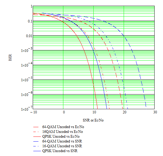
Figure 3 shows the “matched filter bound” theoretical BER performance for uncoded QPSK, 16-QAM, and 64-QAM in AWGN as a function of both SNR, which in this case is equivalent to Es/No, and Ec/No. The curves move along the horizontal scale by a factor of 10log(k) for each modulation as described in Eq. 6. Since this straightforward change in metric makes a significant difference in the locations of the curves, it is always important to select the metric that is best for a given analysis and interpret it accordingly. Mixing different metrics or failing to properly account for the effects of different modulations or code rates or other system differences can make comparisons irrelevant or erroneous.
When FEC is used, as it almost always is, the code rate of the FEC, or the overall code rate of any concatenated FEC systems, needs to be taken into account so that Eb, the payload user information bit energy, is accurately accounted for. Once this is done then the power efficiency of systems with different modulations and FEC systems can be compared independent of data rate or signal bandwidth. As described in Some Observations on Comparing Efficiency in Communication Systems, this is only a power efficiency comparison and does not take into account spectral efficiency or other system characteristics that may be important for overall system tradeoffs. For many systems, however, power efficiency is of sufficient importance that such comparisons may have significant impact on system design and therefore need to be analyzed accurately.
Just as with Es or Ec, the payload bit energy, Eb, can be computed from Ps as follows:
Eb = Ps - 10log(Rb) Eq. 7
Eb = Es - 10log(k) - 10log(R) Eq. 8
where Rbis the payload bit rate and R is the overall FEC code rate with 0 < R
A Handy Compendium of Relevant Relationships
Adjusting the common power efficiency metrics between their various forms can be confusing even for those experienced in their use. Below is a brief compendium of general-case uses for the various metrics discussed above and some examples showing their use.
First, for linear-valued (as opposed to log-scaled) quantities the following relationships hold. Some of these are repeated from above:
SNR = Ps/Pn Eq. 9, Duh.
Es = Ps/Rs Eq. 10, Energy per symbol
Ec = Es/k = Es/log2(M) Eq. 11, Energy per coded bit
Eb = Ps/Rb = Es/(kR) Eq. 12, Energy per payload information bit
No = Pn/BWn Eq. 13
It is often more convenient to work in the logarithmic deciBel scale, and the relationships below can be used when working in dB. Sometimes it is convenient or necessary to switch back and forth between linear and logarithmic scaling, and care should be taken to keep the computations compatible.
SNR = Ps - Pn Eq. 14
Es = Ps - 10log(Rs) Eq. 15, Energy per symbol
Ec = Es - 10log(k) Eq. 16, Energy per coded bit
Eb = Ps - 10log(Rb) Eq. 17, Energy per payload information bit
Eb = Es - 10log(k) - 10log(R) Eq. 18, Energy per payload information bit
Eb/No = Ps - 10log(Rs) - 10log(k) - 10log(R) - Pn + 10log(BWn) Eq. 19, Eb/No in dB
SNR = Eb/No + 10log(Rs) + 10log(k) + 10log(R) - 10log(BWn) Eq. 20, SNR from Eb/No
Examples
A common link configuration for long-range communications uses QPSK modulation with a robust FEC with code rate R = 1/2, so that one payload information bit is encoded in two modulated bits. The net result is that one information bit is transmitted per modulated symbol. For this case, M = 4, k = 2, and R = 1/2. We can then find that:
Eb = Ps -10log(Rs) - 10log(2) - 10log(1/2) = Ps - 10log(Rs) Eq. 21
No = Pn - 10log(BWn) Eq. 22
Eb/No = Ps - 10log(Rs) - Pn + 10log(BWn) Eq. 23
For a matched-filter system BWn = Rs so that for QPSK with R = 1/2:
Eb/No = Ps - Pn Eq. 24
or, more plainly, for this case:
Eb/No = SNR Eq.25
For this special case of a system using matched transmit and receive filters where R is the inverse of k so that there is one payload information bit per symbol, Eq. 25 will hold. This would also be true for R = 1/3 with 8PSK (where k = 3) or R = 1/4 with 16-QAM ( k = 4). While those configurations would not be as practical as the QPSK example, they do illustrate the point.
In a second example grey-coded 16-QAM modulation is used in a simulation with matched transmit and receive filters, and a FEC code rate of R = 5/6. For this case M = 16, k = 4, and R = 5/6. In the simulation only perfectly-synchronized symbol samples are used at baseband with complex-valued AWGN, so that fs = BWn = Rs. For simplicity the sample rate, fs = 1. The following results are computed:
Ps = 99997.1 Eq. 26
Pn = 2522.9 Eq. 27
Es/No = SNR = 15.98 dB Eq. 28
Ec/No = Es/No - 10log(k) = 9.96 dB Eq. 29
Eb/No = Ec/No - 10log(R) = 10.75 dB Eq. 30
As part of the simulation verification process the raw, coded BER was measured with 766 errors in 400400 bits. This would be the BER of the coded bits going into the FEC decoder, yielding BER = 1.913 × 10⁻³. Checking this result against the curves in Fig. 3 we see that the measured BER is on the curves for 16QAM modulation at Ec/No = 9.96 dB and SNR = 15.98 dB. This result gives confidence that the simulation and power metric computations are operating correctly.
Additional Points
Another metric that is sometimes used instead of SNR is C/N, or Carrier-Power to Noise ratio. Often C/No is used to remove dependence on the noise bandwidth. Interpreting C/N or C/No may depend on the type of modulation being used and a clear definition of what was meant by “Carrier Power”. Some modulation types, like the 8-VSB modulation used in the ATSC digital television broadcast standard, use carrier or pilot tones to aid in signal synchronization in the demodulator. For suppressed-carrier modulations like PSK or QAM, however, all of the signal energy is used for modulation of the information. For this reason analyses of PSK and QAM (and other suppressed-carrier modulations) tend to equate SNR and C/N. When residual carrier energy, pilot tones, etc., are present that require energy on their own separate from the modulated data, then care must be taken to be consistent in the use and interpretation of Carrier Power as it relates to Signal Power.
Link budgets, error analysis, simulation, bench testing, and other analyses that require computation or estimation of the various power metric ratios have many pitfalls that routinely frustrate even experienced communication engineers. It is not at all unusual to have a three dB gap between the expected and “measured” performance, and these are commonly due to factor-of-two errors that have crept into the analysis somewhere. Many people have discovered wonderful new signal configurations that result in measured or simulated performance better than expected when compared to theoretical Channel Capacity, only to have their shot at fame dashed by the subsequent discovery of an error in calibrating or computing their power metrics. A few simple sanity checks may help find errors in computing power metrics before they are able to cause too much confusion. Generally, keeping track of whether computed quantities should grow or shrink compared to other metrics can go a long way to nip errors in the bud. The following are suggestions for simple sanity checks:
Es < Ps as long as the symbol rate is greater than 1 Hz,
Ec < Es for modulation orders having greater than 1 bit/symbol
Since FEC code rates are always less than one, unless the system is uncoded so that R = 1:
Ec < Eb whenever FEC is used,
Ec = Eb when the system is uncoded.
Eb < Es except for uncoded BPSK or other modulations with one bit per symbol.
No < Pn as long as the noise bandwidth, BWn, is greater than 1 Hz.
Conclusion
Power metrics and power metric ratios provide means for evaluating and comparing system performances in various contexts. A variety of metrics are available as analytic tools but must be carefully and properly applied in order to obtain accurate and useful results. Some of the most common metrics and their use and limitations are described above, as well as some examples and methods for basic sanity checks. While pitfalls and mistakes in the use of these metrics are not unusual they may be minimized or avoided by better understanding and careful checking of results. This article attempts to provide a basis for basic understanding of the metrics discussed as well as their use, limitations, and some simple methods for self-checking.
List of Terms
| AWGN | Additive White Gaussian Noise. This is the common model for thermal noise. |
| C | Carrier power. For suppressed carrier systems like PSK, QAM, and MSK this is generally interchangeable with total signal power. |
| Ps | Total signal power. This is the S in SNR. |
| Es | Energy per symbol. This is the total signal power divided by the symbol rate, Rs. |
| Ec | Energy in a single coded bit, or bit into the FEC decoder. Ec is related to Es by the modulation type, specifically the number of coded bits per symbol, k. |
| Eb | Energy in a single payload information bit, or bit out of the FEC decoder. This is the total signal power divided by the information bit rate, or Ec divided by the FEC code rate, R. |
| N | Noise power. This is the total noise power in a system and is the N in SNR. |
| Pn | Also the total noise power, but often used as the amount of noise power measured in a given test. |
|
No |
The noise power in a unit Hz bandwidth. This is the total noise power divided by the bandwidth of the noise. This may be tricky to determine if the noise density is not constant across all frequencies. |
| BW | Bandwidth. Often no subscript indicates that the signal bandwidth is implied. |
| BWn | Noise bandwidth. In a calibrated noise bench test this number may be adjusted to account for the shape of the noise spectrum to provide the normalized noise bandwidth. In a simulation this is usually proportional to the assumed sampling rate. |
| R | The FEC code rate, such that Rb/Rc = R. For most purposes this is the overall FEC code rate including all concatenated codes if so used. |
| Rs | Symbol rate. |
| Rc | Coded bit rate. This is the bit rate into the FEC or kEc |
| Rb | The payload information bit rate. This is the data rate out of the FEC. |
| M | The order of the modulation type. e.g., M = 2 for QPSK, M = 64 for 64-QAM. |
| k | The number of bits per modulated symbol. k = log2(M) and M = 2k. |
References
[1] J. B. Johnson, “Thermal Agitation of Electricity in Conductors”, The American Physical Society, 1928.


- Comments
- Write a Comment Select to add a comment
Continue your awesome work, Eric!
To post reply to a comment, click on the 'reply' button attached to each comment. To post a new comment (not a reply to a comment) check out the 'Write a Comment' tab at the top of the comments.
Please login (on the right) if you already have an account on this platform.
Otherwise, please use this form to register (free) an join one of the largest online community for Electrical/Embedded/DSP/FPGA/ML engineers:


