Time-Domain Periodicity and the Discrete Fourier Transform

• DFT_FFT

Introduction

The Discrete Fourier Transform (DFT) and it's fast-algorithm implementation, the Fast Fourier Transform (FFT), are fundamental tools for processing and analysis of digital signals. While the continuous Fourier Transform and its inverse integrate over all time from minus infinity to plus infinity, and all frequencies from minus infinity to plus infinity, practical application of its discrete cousins can only be made over finite time and frequency intervals. The discrete nature and finite support region of the DFT creates effects on the output characteristics that must be understood in order to properly interpret the results.

The cyclic nature of the repeating spectrum of sampled signals is fundamental and well understood by most practitioners of signal processing. The "aliasing" behavior of energy sampled in discrete time is conceptually important and can be exploited to significant advantage when properly understood. Likewise the frequency-domain response of tones that are not only sampled in discrete time but are observed over a finite window of time exhibit consistent behavior that is sometimes non-intuitive and frequently misunderstood. In this article we attempt to show that different points of view of conceptual processing models of the DFT are consistent with each other and each provides significant insight into signal behavior and interpretation of DFT outputs. This provides the user with different options of conceptual models to use to understand, predict, and process signal responses when using the DFT and its related processes.

Time Windows

All practical, real-world, signals are observed over finite periods of time. This fact alone moves us a step away from the elegant, ideal mathematical model of the continuous-time Fourier Transform (CTFT) when dealing with practical signals. While the CTFT provides an important and useful analytical tool, the differences between it and the application of finite-support discrete-time Fourier Transform (DTFT) or DFT operations are significant. In this article we focus on the DFT and FFT since they are the tools most frequently used in practical algorithm implementations.

A critical concept in fully understanding the output behavior of a DFT hinges on the Convolution Theorem, which says that convolution in the time domain corresponds to multiplication in the frequency domain. This can be expressed as:

         h(t)*x(t) <> H(f) X(f)          Eq. 1

where * denotes convolution, <> indicates a domain transformation, and x(t), X(f) are Fourier Transform pairs. Likewise, and importantly for the purposes of this article, the converse is also true so that multiplication in the time domain corresponds to convolution in the frequency domain, expressed as:

         h(t) x(t) <> H(f)*X(f)          Eq. 2

This theorem applies to the frequency analysis of any finite-time signal or series since the application of an observation window to a signal is effectively multiplication by a rectangular function that is unity during the observation time and zero everywhere else. This is essentially the classic case of a rectangular window being applied to the time-domain sequence. The result is that the frequency-domain profile of the signal, when processed with a forward FT of length equal to or longer than the length of the time observation window, is effectively convolved with the Fourier transform of the time-domain observation window. This is true whether the window is rectangular or has some other shape that is applied independent of the signal content.

Letting x(t) be the time domain sequence and h(t) be the arbitrary window function in the time domain, Eq. 2 indicates the general behavior of the transform. If h(t) is a rectangular function then H(f) is the familiar sin(x)/x shape with main lobe width and sidelobe spacing dictated by the time length of the rectangle (Eq. 3, Fig. 1). Generally the 3-dB width of the main lobe of H(f) is used to determine the frequency-domain "resolution" of the analysis provided with that particular window function. The longer the observation time, the narrower the main lobe of the frequency-domain response and the better the frequency "resolution", or ability to accurately estimate frequency or separate two tones. This is essentially the basis for the time-frequency "uncertainty principle" in signal analysis, since it is not possible to have full resolution in the frequency domain without an infinitely long observation period in time, or in the time domain without knowledge of the frequency domain from minus to plus infinity.

         h(t) = A(-T₀, T₀) <> H(f) = 2AT₀ sin(2πT₀f)/(2πT₀f)          Eq. 3

Note that Equations 1, 2, and 3 are general and are expressed in terms of continuous-time functions and transform pairs with the CTFT. Their application is not limited to the DFT, but they apply directly to it since the time- and frequency-domain support of the DFT are both finite. For the discrete-time case the length of the rectangular function becomes 2T₀ = nT_s, and the spacing between nulls in the sin(x)/x function is then 1/nT_s = (N/n)(f_s/N) where N is the length of the DFT. The sampling period in the time domain is T_s and therefore the bin spacing in the frequency domain is f_s/N with 1/T_s = f_s. For the case shown in Fig. 1, N = 256, the time-domain pulse has length n = 10 samples, and it can be seen that the length-N DFT output has n = 10 nulls evenly spaced on both sides of the sin(x)/x main lobe. The generality of Eq. 3 means that the nulls of the sin(x)/x in the frequency domain due to the window function will always be spaced at N/n for a length-n window, and if the window is the entire length of the transform then the nulls are N/N = 1 bin apart. If the main lobe of the sin(x)/x is exactly centered in an output frequency bin, i.e., there is exactly an integer number of cycles of the tone in the length-N DFT input aperture, then the rest of the output samples will fall exactly on the nulls of the sin(x)/x and will contain no energy due to that tone. This does not mean that the sin(x)/x sidelobes do not exist, they are just between the output samples of the DFT. If there is a non-integer number of cycles of a tone in the DFT input, then the peak of the main lobe of the sin(x)/x will not be in a bin center and the adjacent output samples will fall on the sidelobes rather than on the nulls. Figure 2 illustrates this difference.

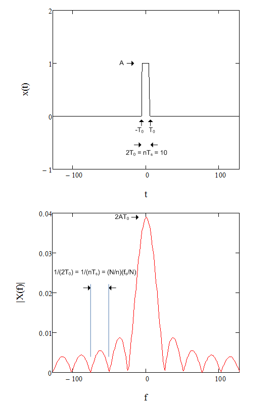
Figure 1. Shown is the Fourier Transform pair for a rectangular pulse in the time domain (upper plot) with a sin(x)/x function in the frequency domain (lower plot) that corresponds to Eq. 3. For the discrete-time case a pulse of length n samples results in nulls spaced N/n bins apart.

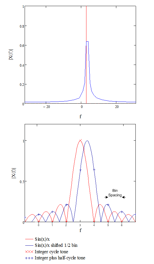
Figure 2. The frequency-domain sampling of the sin(x)/x response of a rectangular window of the length of the transform is shown for the case with an integer number of cycles (red) and the same number of cycles plus an additional half cycle (blue). In the upper plot there are exactly three cycles in the aperture for the red case, and three and a half for the blue trace. In the lower plot the sin(x)/x response in between the bin samples is shown for both cases.

An example case is shown in Figure 2. In Fig. 2 the red trace is the DFT output magnitude for the case of exactly three cycles of a complex sinusoid in the length-N DFT input. In other words the input frequency is exactly f = 3/NT_s. This places the peak of the sin(x)/x response due to the length-N input window exactly at bin 3, with the nulls between the sidelobes falling exactly on the remaining output bin samples, as shown in the lower plot of Fig. 2.

If the frequency of the input signal is increased so that there are exactly three and one-half cycles within the full length-N DFT input, so that f = 3.5/NT_s, the sin(x)/x moves one-half output bin, halfway between bins 3 and 4, so that the main lobe is sampled on both sides and the sidelobes are sampled half-way between each null. This is shown by the blue trace in Fig. 2, with the plus-sign markers showing the locations of the output samples in the lower plot. The effect is that the envelope of the sin(x)/x becomes the output of a magnitude display as shown in the upper plot of Fig 2. Note that the only change in the input is an increase of frequency of one-half cycle over the full length-N input of the DFT, but the output magnitude responses appears to change significantly in the upper plot. The behavior is fully explained by the convolution of the ideal output spike at the input frequency and the sin(x)/x Fourier transform of a rectangular window of the full length of the DFT.

The finite-length input "window" of the DFT is often called the "aperture", since it is essentially the window or opening through which the DFT "sees" the input. This is analogous to the aperture of a camera or optical system and shares some of the same properties, e.g., the output resolution improves with the increasing size of the aperture.

Periodicity and Alternative Conceptualizations

What's outside of the input window or aperture has no affect on the output of the DFT since those input samples, if they exist, are not used in the computation of the output. Figure 3 shows three different cases where a length n = 64 window is applied to different input sequences, with the samples within the window identical in all three cases. Since these finite-length input sequences within the indicated windows (shown by the dashed vertical markers) are identical in all three cases their DFT outputs will also be identical in all three cases. The common windowed signal shown consists of exactly three-and-a-half cycles of a complex sinusoid, matching the cases shown by the blue traces in Fig. 2. In the first case shown in Fig. 3, x1_n, the full sequence is a continuous tone and the window applied to a segment of that. In the second case, x2_n, the sequence of three-and-a-half cycles of the tone is repeated continuously, so that every 64 samples there is a phase discontinuity of π radians. In the third case, x3_n, there is Gaussian noise everywhere outside of the window region.

Since the windowed portions of all three sequences shown in Fig. 3 are identical, their DFT outputs will be identical and indistinguishable from each other in that sense. This raises an important point in that the DFT of a sequence is relevant only to that sequence and contains no information at all about any other part of the input stream outside of the DFT aperture. Nevertheless, careful consideration of the three cases shown can be used to gain some insight into the general behavior and interpretation of the DFT. There are alternative

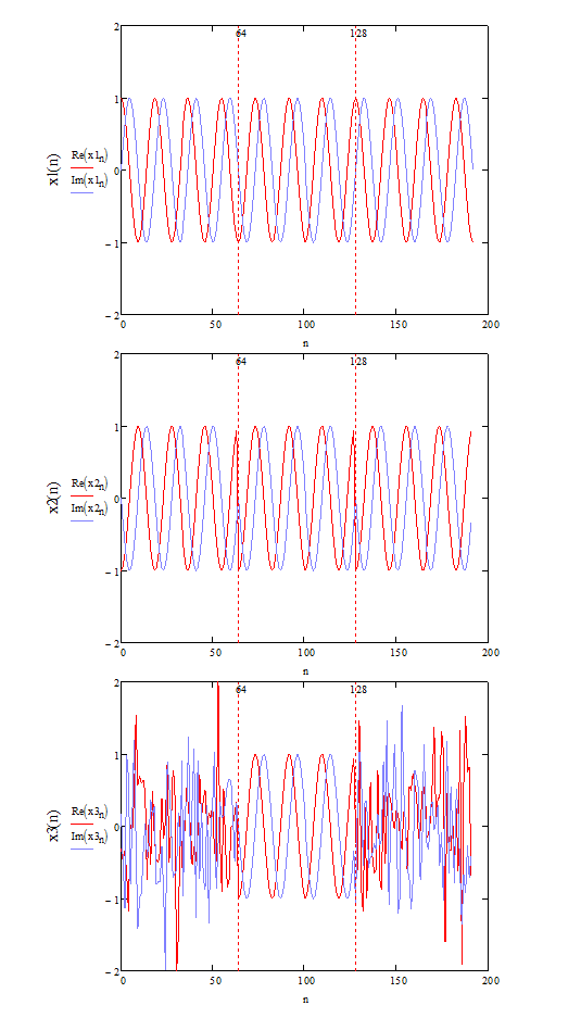
Figure 3. Shown are three time-domain signals that have the same DFT output when the input is taken from the window region between the dashed vertical markers shown. In the first the signal, x1_n, is a continuous complex sinusoidal wave, in the second, x2_n, the sequence repeats the non-integer number of cycles that appear within the window, and in the third, x3_n, the signal outside of the window region is Gaussian white noise.

points of view or interpretations that can be taken to explain the behavior of the DFT with respect to the visibility of the sin(x)/x sidelobes as shown in Fig. 2. Many of the theoretically inclined often use a point of view relevant to x2_n in Fig. 3, where the input is considered to be an infinitely repeating sequence with period equal to the DFT length. In this case the input window can be considered to conceptually disappear, since the frequency content of the extended sequence is the same as the frequency content of the windowed sequence, with frequencies other than the fundamental introduced due to the periodic phase discontinuity at the ends of the DFT aperture. This viewpoint is sometimes preferred since it is more closely conceptually consistent with the continuous-time Fourier Transform and therefore the analytical treatment lends itself to the use of the CTFT. Likewise the behavior of the DFT in this viewpoint is consistent with the behavior of the CTFT of the periodically repeating input sequence, with the DFT outputs equal to the values of the CTFT of the periodically repeating input at the frequencies sampled by the DFT.

Some folks err, however, in a common misconception that the interpretation of the DFT output is only proper for the point of view considering the input to be a periodically repeating sequence. Fig. 3 helps illustrate this, in that the cases shown and their transform as the blue traces in Fig. 2 are fully consistent, analytically and conceptually, with the windowed input point of view previously described. Both points of view are useful and correct in their own context. It is especially helpful that if one of the points of view seems conceptually difficult then the other can be used to help properly interpret and understand DFT output sequences. Understanding both points of view provides the broadest potential for properly interpreting DFT outputs. It is somewhat elegant and aesthetically pleasing that while both points of view are conceptually different they are both consistent with the theory and behavior of the DFT and consistently explain its output.

Zero-Padding

An important related application topic, while already formally addressed in the Time Windows section, is zero padding. Zero padding a DFT input essentially shortens the length of the rectangular window function applied to the DFT input without changing the length of the DFT. For a length-N DFT this provides N output bins with a spacing of 1/NT_s with a resolution related to the width of the sin(x)/x main lobe due to the length of the non-zero portion of the input sequence, less than N, and as shown in Figure 1. This stresses the point that the frequency resolution due to the main-lobe width of the frequency impulse response is determined by the observation time, i.e., the length of the effective time-domain window, and the output frequency bin spacing is determined by the sampling period of the input sequence. The output bin spacing and the 3dB main-lobe width of the sin(x)/x frequency response are only the same when the input sequence window is the same as the length of the DFT, and generally when the window is rectangular.

Zero-padding is sometimes applied to achieve DFT output bin spacing of 1/NT_s, or to use an available length-N FFT routine or core, when N input samples may not be available. It may also be used in some cases to reduce computational complexity since computations associated with the zero-valued input samples can be skipped. Usually zero-padding is accomplished by filling the input array starting at the first element and inserting zeros from the end of the sampled data to the end of the DFT input array. Figure 4 shows a case where the data is placed near the center of the input vector and zeros are padded before and after the data to fill the rest of the input array. Moving the data window earlier or later in the time domain aperture of the DFT exposes the non-zero data window to different phases of the DFT basis functions, as shown in the middle plot of Fig. 4. The Bin 1 Basis Function shown in Fig. 4 is the basis function related to the DFT output index k = 1, with one cycle of the complex sinusoid basis function over the full length of the DFT. It can be seen that moving the non-zero data window earlier or later results in a phase change, which is consistent with the Time-Shifting property of the DFT shown in Eq. 4. Since the absolute phase of the DFT output is usually, but certainly not always, inconsequential to many applications this phase change is often not important so that aligning the data window with the beginning of the DFT input aperture is often the simplest and most straightforward approach.

         h(t - t₀) <> H(f)e^-j2πft₀          Eq. 4

Also shown in Fig. 4 is the magnitude of the DFT output for the zero-padded input shown. Since the input signal contains a complex sinusoid with a period equal to exactly one-fifth of the length of the full DFT aperture, the peak of the output sin(x)/x response will be centered in output bin number five, i.e., k = 5. The width of the main lobe of the sin(x)x and the sidelobe null spacing is determined strictly by the length of the input window. In this case the input window is exactly one-fifth of the length of the DFT input aperture, so the output sidelobe nulls will be five bins apart. The red trace in the plot of |X4(k)| in Fig. 4 shows the DFT of the continuous input tone of the same frequency if the window were the full length of the DFT input.

Conclusion

Interpretation of DFT outputs can be confusing if one is not aware of the effects of the finite-length and the resulting sin(x)/x frequency response. The response and its effect on the output can be easily predicted and understood from multiple viewpoints: first as a convolution of the signal frequency content within the finite-length window and the frequency transform of the window, and second as the transform of an infinitely repeating sequence with period equal to the length of the transform. Either approach is useful for explaining and understanding the behavior of the DFT.

Many of the common questions and pitfalls associated with interpreting DFT outputs can be explained by the effects of the sin(x)/x output response due to the finite-length input. The frequency-dependent presence, absence, or magnitude of sidelobe energy often leads to an assessment of a bug or error in the process when no bug exists. An alternate interpretation, where the input sequence is treated as a single period of an infinitely repeating signal, is also consistent with theory and more closely conceptually consistent with the Continuous-Time-Fourier-Transform. Either approach can be used to understand and interpret DFT outputs when analyzing or processing discrete-time sampled signals.

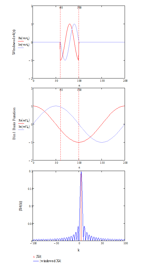
Figure 4. Zero-padding of the input is often used to match the length of an input sequence with the length of an available FFT routine or core. The effect is the same as shown in Fig. 1 in that the length of the effective data window determines the breadth of the sin(x)/x response in the frequency domain. Since the basis functions are matched to the length of the DFT and not the length of the data window, sliding the data window within the DFT input aperture changes the phase relative to the DFT basis functions.

References

[1] E. Oran Brigham, The Fast Fourier Transform, Prentice-Hall, Englewood Cliffs, NJ, 1974
[2] Richard G. Lyons, Understanding Digital Signal Processing, Prentice-Hall, 3rd Ed., 2010
[3] Alan V. Oppenheim, Ronald W. Schafer, Digital Signal Processing, Prentice-Hall, 1975
[4] John G. Proakis, Dimitris K., Manolakis, Digital Signal Processing, Prentice-Hall, 4th Ed., 2006

Sign in