Frequency-Domain Periodicity and the Discrete Fourier Transform

• DFT_FFT

Introduction

Some of the better understood aspects of time-sampled systems are the limitations and requirements imposed by the Nyquist sampling theorem [1]. Somewhat less understood is the periodic nature of the spectra of sampled signals. This article provides some insights into sampling that not only explain the periodic nature of the sampled spectrum, but aliasing, bandlimited sampling, and the so-called "super-Nyquist" or IF sampling. The approaches taken here include both mathematical and intuitive treatments in order to provide the basis for a broad understanding of the topic for those inclined to either method.

For Digital Signal Processing the relevant tool of interest is usually the Discrete Fourier Transform (DFT) or its quicker cousin the Fast Fourier Transform (FFT), and an understanding of the general ideas of sampling and aliasing is critical to proper application of those tools. The concepts demonstrated in this article are intended to aid in understanding the realities of the mechanisms behind the requirements of the Nyquist sampling theorem, and will also help explain the circular and periodic nature of the spectra of sampled signals.

Throughout this article both the mathematical and intuitive treatments are made assuming complex-valued signals and arithmetic, so that the maximum signal bandwidth for alias-free reconstruction of the sampled signals is the sampling frequency, f_s, rather than f_s/2, as it would be for real-valued signals. This is possible since each complex sample is composed of two independent samples, one each for the real and imaginary (or quadrature) components, so Nyquist is not violated.

We delve into the mathematical analysis first, so feel free to skip that if you think it'll make your head hurt and you want to go straight to the intuitive treatment. If I were reading this on my own that's probably what I'd do. ;)

First, The Math

Many mathematical treatments of periodic discrete-time sampling that address the periodic spectrum make reference to the Poisson Summation Formula or just state that if a time series is periodic over period N then the spectrum will also be periodic over N samples. These approaches generally make the assumption that the sampled time sequence is periodic over N samples for convenience in order to make the math work out more easily. Exact periodicity over N samples of interest is rarely the case in practical applications and most real-world signals are better represented in a stochastic sense than with assumptions of exact periodicity over any given set of samples. The assumption of periodicity in the time-domain over N samples therefore creates a disconnect between theory and most practical applications.

In Oppenheim and Schafer's Discrete-Time Signal Processing [5], another approach is used which does not make any assumptions of signal periodicity and still reaches a reasonably rigorous conclusion with a periodically repeating spectrum. This provides a more general solution for those who are uncomfortable with processing non-periodic signals using interpretations based on periodic input assumptions. The argument starts with the definition of a sampling impulse train s(t) as:

where δ is the unit impulse function or Dirac delta function and T is the sampling period. The discrete-time sampling of the continuous-time signal x_c(t) is then

where x_s(t) is the discrete-time sampled version of x_c(t). Since x_s(t) is the product of the continuous-time signal x_c(t) and the sampling impulse train s(t), the Fourier transform of x_s(t) is the convolution of the Fourier transforms of x_c(t) and s(t). The Fourier transform of a periodic impulse train is also a periodic impulse train with period equal to the sampling frequency [6][8]. The result is that the Fourier transform of Eq. 2 is then, using notation consistent with O&S,

where Ω_s = 2π/T is the sampling frequency in radians/second. Note that Eq. 3 shows that the spectrum of x_s(t) contains the spectrum of x_c(t), specifically X_c(jΩ), repeating infinitely at intervals equal to the sampling rate. Note also that this is a general result with no assumptions regarding the periodicity, content, or bandwidth of x_c(t). If the spectrum of x_c(t) has greater bandwidth than the sampling frequency, the repeating spectra, X_c(jΩ), will overlap and aliasing will occur in the discrete-time sequence x_s(t).

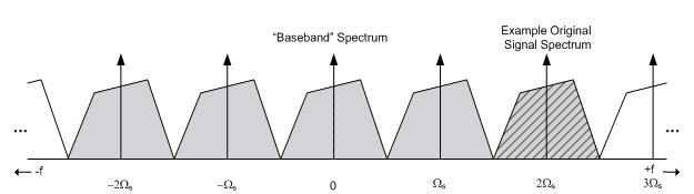
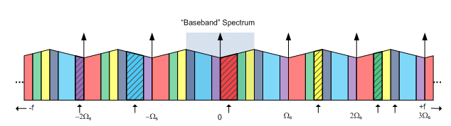
If x_c(t) is bandlimited with bandwidth, B, less than the sampling rate, Ω_s, then X_c(jΩ) will not overlap when repeated in X_s(jΩ) and x_s(t) will not contain aliased energy and can be used to reconstruct x_c(t) using a bandlimiting filter. Note that the bandlimited spectral energy of x_c(t) can be located anywhere in the frequency domain from minus to plus infinity. The only restriction to avoid aliasing is that its bandwidth be limited to less than Ω_s in order to prevent overlap of the replicated spectra. This is consistent with the Nyquist sampling criterion. Figure 1 shows an example of a repeating non-overlapping bandlimited signal spectrum with the replicas centered on integer multiples of the sampling frequency. This is the traditional arrangement that results in the complex-valued, asymmetric spectrum of interest at "baseband" straddling zero frequency. The spectrum of the original example bandlimited signal, x_c(t), could be represented by any one of the infinite number of replicas and the repeating spectrum shown would be the spectrum of the resulting discrete-time sampled signal, x_s(t).

Oppenheim and Schafer also show in [5] that the Discrete-Time Fourier Transform (DTFT) of the system described above can be arrived at without loss of generality as a rescaling process that is consistent with the sampling characteristics and conventions used for digital signals. Since the sampled domain spacing of a digital signal's samples is unity, which may include a time scale of the sampling period, T, for a time-domain signal, and to support the traditional convention of the sampling frequency Ω_s = 2π, then a rescaling factor in the "frequency" domain of ω = ΩT can be applied starting with the definition of the DTFT:

then

where X(ω) is the DTFT of x_n = x_c(nT). Combining Eqs. 3 and 5 then yields:

which is the infinitely repeating spectrum of x_c(t) spaced at 2π radians/sample instead of Ω_s radians/sec.

A simple additional step can be made by observing that if a length-N rectangular window is placed on a segment of x_n = x_c(nT), then the summation of the DTFT in Eq. 4 can be limited to n = 0..N-1. Evaluating X(ω) in Eq. 4 at the discrete frequencies ω = 2πm/N then transforms Eq. 4 into the DFT, X_m, of x_n = x_c(nT). The frequency index m can run over any range, just like ω, but will result in redundant computations if extended beyond one interval of the sampling rate, Ω_s = 2π/T, as described in Eq. 6 and as shown in Fig. 1. Traditionally m is then restricted to m = 0..N-1 or, alternatively, m = -N/2..N/2-1 to select the "baseband" spectrum including zero frequency. Again, the computation of the DFT as described is consistent with the previous analysis and loses no generality. The application of the rectangular window to x_n to limit the length of the processed sequence requires no assumptions about the periodicity of the original signal, x_c(t), and also fully explains the sin(x)/x response in the frequency domain [7].

The Intuitive Approach

For the non-math geeks (like me) there is, fortunately, an intuitive method that also fully illuminates the mysteries of the repeating spectrum of sampled systems, aliasing, and the so-called "super-Nyquist" sampling which is sometimes also called IF sampling (for Intermediate Frequency) or bandpass sampling. Many are familiar with the "wagon wheel effect" where the spokes of a wheel appear to turn backward or at a rate that clearly does not match the speed of the vehicle. This is essentially an example of aliasing where the sampling is typically at the frame rate of the video display, or, sometimes, the rate of flicker of artificial lighting (e.g., 120 Hz in the US, 100 Hz in Europe). Some physics classes include either demonstrations or lab experiment assignments using a stroboscopic light and a spinning wheel or similar apparatus to provide a hands-on method of examining the phenomenon.

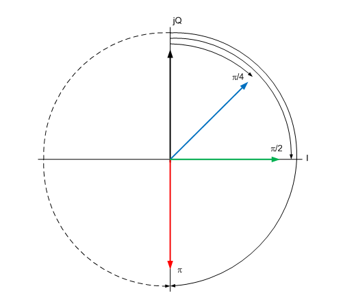
Since a complex-valued signal can be thought of as a vector in the two-dimensional complex plane with a magnitude and phase, the same mechanisms that create the "wagon wheel effect" can be examined in the case of a vector rotating at a constant rate with a constant magnitude, in other words, a complex sinusoid. Figure 2 shows a complex plane with four different vectors, with the black vector representing an initial reference sample from which rotation will be measured to the next sample in time. If there is no rotation, the next sample and every subsequent sample will be in the same location as the black vector. If the next sample taken is the blue vector, then the phase is advancing at a rate of π/4 radians/sample; if it is the green vector then π/2 radians/sample; and the red vector, π radians/sample.

The red vector reveals an ambiguity in that a rotation between samples of π radians (clockwise) cannot be distinguished from a rotation of -π radians (counter-clockwise). This is the case where the signal frequency is exactly at half of the sampling frequency, and is why many state the Nyquist sampling theorem for baseband signals as requiring sampling higher than twice the highest signal frequency rather than equal to it. One way of removing the ambiguity in the supported frequency interval is to state that for a system sampled at frequency Ω_s = 2π the baseband interval is [-π,π) rather than (-π, π), and this is often done in authoritative texts. This suggests that if there is signal energy at -π that the rotation is counterclockwise rather than clockwise, when the reality is that the two are indistinguishable and an unresolvable ambiguity exists. Stating the interval as [-π,π) rather than (-π, π) removes the ambiguity in the math and makes the analysis cleaner (and tractable), but does not allow one to distinguish the direction of rotation of a physical system or complex signal with samples measured at π or -π radians/sample.

Additional ambiguities lurk, too. Even if the black vector is the result of sampling at every sample instant, the vector could be stationary or could be rotating at integer multiples of full rotations between every sample either clockwise or counterclockwise. So the possible frequencies of the input signal represented by two adjacent time samples of an unchanging vector are ω = n2π, with n being any integer, including zero for the stationary case. Likewise the blue vector could represent a frequency of π/4 or -7/4π radians/sample, or any integer number of full rotations plus those quantities. Figure 3 shows the spectrum of the possible frequencies for each case. The black spikes are the possible frequencies for the case where there appears to be no rotation from one sample to the next, the blue spikes correspond to the blue vector in Fig. 2, as do the other colored spikes. The red spikes occupy the "Nyquist frequency", or the so-called "folding frequency" at exactly half of the sample rate.

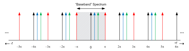
Comparison of Figures 1 and 3 show the consistency between the mathematical and intuitive explanations provided here. Since Figure 1 represents the CTFT of a discrete-time sampled sequence the sampled spectrum is shown on a continuous frequency axis with the replicated input spectra centered on multiples of the sampling frequency, Ω_s. In Figure 3 the spectrum is shown more generally and the horizontal axis is simply radians/sample, so that the samples could have been taken across time or space or any other dimension. The mathematical and intuitive analyses both reveal periodic, infinitely repeating spectra with period equal to the sampling rate.

Slightly More Advanced Topics

The repeated periods of the spectral content represent ambiguity regions that are indistinguishable from each other in a sampled system. Removal of the frequency ambiguities in a practical system involves eliminating all possible ambiguity regions but one for each possible frequency prior to sampling. Typically this is done with low-pass analog anti-alias filters prior to the sampler (e.g., ADC) that eliminate energy from all of the ambiguity regions except the baseband region below half the sampling frequency. For some systems, sometimes systems measuring signals at radio frequencies, it is beneficial and practical to isolate one of the ambiguity regions at higher frequencies beyond the baseband region, typically using an Intermediate Frequency filtered with a bandpass filter. High-Q bandpass filters, like SAW or other resonant filters, provide enough isolation to eliminate enough energy from all the other ambiguity regions for successful sampling and reproduction of the desired signal. This is the case shown in Fig. 1, where the input signal energy is centered at 2Ω_s. The frequency-periodic nature of sampling then allows the signal to be processed as though it originally existed at baseband, potentially eliminating a mixing step in the system.

The sampled-IF case demonstrates why many are careful to quote the Nyquist sampling theorem as referring to the bandwidth of the signal rather than the highest frequency content. Strictly speaking the input frequency can be anything, but if the total bandwidth of the continuous signal exceeds half the sampling frequency for real-valued signals (or the sampling frequency for complex-valued signals) then unresolvable frequency ambiguities will exist where the repeated spectra overlap. Sampled-IF systems work by keeping the sampled signal bandwidth within the requirements of the Nyquist sampling criterion, even though the signal frequencies are well outside the baseband region and potentially even above the sampling frequency.

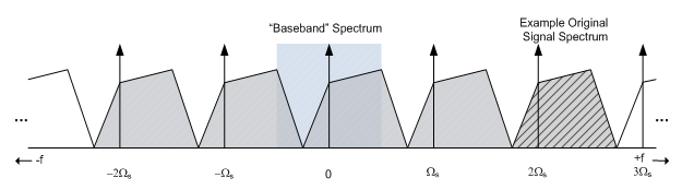
It is useful to note that it is not even necessary to keep the signal energy within one ambiguity region in the frequency domain. Figure 4 shows a case where the input signal is not centered on a multiple of the sampling frequency and spills over into an adjacent ambiguity region. Since the spectrum is periodic this makes such a shift appear as a cyclic shift in the baseband region. Even though some of the energy in the baseband region appears as though it "aliased" in from the adjacent spectral replica, mixing the sampled baseband signal with a complex sinusoid of the appropriate frequency can shift the entire spectrum, including all of the replicas, back to the condition shown in Figure 1 if so desired. This will appear as cyclic shift at baseband with the energy shifted out on the left side of the baseband region shifting in on the right side. Since the signal still meets the Nyquist criterion of not exceeding the bandwidth supported by the sample rate, the original signal can be fully reconstructed even though it is not fully contained within one of the spectral ambiguity regions.

An additional and slightly more obscure point is that not only can the continuous input signal spectrum straddle two ambiguity regions, it can potentially be scattered across an infinite number of them and still be recovered without ambiguity or aliasing. Figure 5 shows an arrangement whereby bands from five different ambiguity regions are occupied by input signal energy as indicated by the bolded and striped regions with arrows below. Since the replicas of the striped input regions do not overlap each other, the signal can be reconstructed if the original input frequencies are known. Figure 3 can be used to illustrate the same concept if each of the colored spikes was due to an input tone in a different ambiguity region. As long as the colored regions in Fig. 4 don't overlap each other, then it will be possible to resolve which ambiguity region the baseband energy came from. This could be accomplished with careful isolation of the striped regions with individual bandpass anti-aliasing filters prior to the sampler but this is not a trivial undertaking. The system as shown in Fig. 4 is not symmetric about zero frequency and therefore implies that the input signals are complex-valued at the input to the sampling system. This could be accomplished with a block converter that moves a band much greater than the sample rate to baseband with a complex-valued output.

Conclusion

The periodic nature of the spectra of sampled signals can be understood from both mathematical and intuitive foundations. When extended to the DFT or FFT the mathematical basis for the periodic replication of signal spectra in sampled systems is often presented as requiring periodicity in the time domain with period equal to the length of the transform input. Such treatments are often done for convenience and simplicity and a more general approach which does not require an assumption of input periodicity has been shown here with the basis of the approach taken from [5]. An intuitive approach was also presented which demonstrates the same properties as the mathematical approach without requiring understanding of anything beyond the basics of the sampling process.

Once a basic understanding of the mechanisms behind the frequency-domain periodicity is obtained it is then also possible to understand more advanced sampling techniques. The so-called "super-Nyquist" or "sampled-IF" technique was explained as well as the potential to simultaneously use multiple input bands spread across many multiples of the sample rate.

While many may think of the frequency-domain periodicity and cyclic nature of the DTFT, DFT, and FFT as difficult conceptual burdens or hurdles, it allows exploitation of various techniques that may allow significant simplification in practical systems. Sampled-IF systems have been fairly common in communication systems for several decades and requirements for low power consumption may drive more systems to use sample rates lower than the signal frequency or exploit other interesting sampling tricks. The invention of paradigm-shifting technologies based on these ideas is left to the reader with the author's request to be remembered with warm thoughts, cold beer, or other valuable consideration should one manage to pull that off. ;)

References

[1] H. Nyquist, "Certain topics in telegraph transmission theory", Trans. AIEE, vol. 47, pp. 617–644, Apr. 1928 Reprint as classic paper in: Proc. IEEE, Vol. 90, No. 2, Feb 2002
[2] Richard G. Lyons, Understanding Digital Signal Processing, Prentice-Hall, 3rd Ed., 2011
[3] Alan V. Oppenheim, Ronald W. Schafer, Digital Signal Processing, Prentice-Hall, 1975
[4] John G. Proakis, Dimitris K., Manolakis, Digital Signal Processing, Prentice-Hall, 4th Ed., 2006
[5] Alan V. Oppenheim, Ronald W. Schafer, Discrete-Time Signal Processing, Prentice-Hall, 1989
[6] Alan V. Oppenheim, Alan S. Willsky, Signals & Systems, Prentice-Hall, 2nd Ed., 1996
[7] Eric Jacobsen, "Time-Domain Periodicity and The DFT", dsprelated.com, July, 2012
[8] E. Oran Brigham, The Fast Fourier Transform, Prentice-Hall, Englewood Cliff_s, NJ, 1974

Sign in