Setting the 3-dB Cutoff Frequency of an Exponential Averager

• Tips and Tricks

This blog discusses two ways to determine an exponential averager's weighting factor so that the averager has a given 3-dB cutoff frequency. Here we assume the reader is familiar with exponential averaging lowpass filters, also called a "leaky integrators", to reduce noise fluctuations that contaminate constant-amplitude signal measurements. Exponential averagers are useful because they allow us to implement lowpass filtering at a low computational workload per output sample.

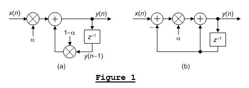
Figure 1 shows two, a two-multiply and a one-multiply [1,2], exponential averagers. Given the same value for the α weighting factor, the two averagers have identical performance.

WEIGHTING FACTOR APPROXIMATION FORMULA
Years ago I was introduced to the following expression for computing the α weighting factor to set an averager's 3-dB cutoff frequency to f_c Hz:

where f_s is the averager's input data sample rate in Hz [1]. The “app” subscript in Eq. (1) stands for approximation. I did some Matlab modeling of Eq. (1) and found it to be useful so long as f_c was less than roughly 0.1f_s. I hadn't thought much more about Eq. (1) after that, thinking that it was a little-known approximation formula. However, I recently received an E-mail from a signal processing engineer asking why I didn't include Eq. (1) in the 'Averaging' chapter of my DSP book. So perhaps Eq. (1) is more widely known than I thought. That E-mail convinced me that it might be useful to write a short blog on how to design an exponential averager with a given 3-dB cutoff frequency.

EXACT WEIGHTING FACTOR FORMULA
The correct expression for computing the α weighting factor to set an exponential averager's 3-dB cutoff frequency to f_c Hz is [3]:

The “cor” subscript in Eq. (2) stands for correct. The derivation of the messy Eq. (2) is given in the Appendix.

So the question is, “What is the error in using the α_app approximate weighting factor for various values of the 3-dB cutoff frequency f_c?” Figure 2 shows the frequency magnitude and phase responses of two exponential averagers when the f_c cutoff frequency is one tenth of the f_s sample rate. The solid blue curves correspond to a correct α_cor computed using Eq. (2). The dashed red curves correspond to an α_app computed using Eq. (1).

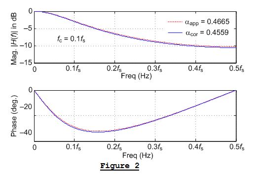
The solid blue α_cor magnitude curve in Figure 2 has the desired -3 dB value at f_c = 0.1f_s Hz. The dashed red α_app magnitude curve's value at f_c Hz is -2.86 dB. So at such a low value of f_c, the two magnitude curves are quite similar and Eq. (1) is an acceptable approximation to Eq. (2).

When we set f_c = 0.2f_s Hz, on the other hand, Eq. (1)'s α_app falls short on performance. Figure 3 shows the performance of the two exponential averagers when f_c = 0.2f_s Hz. The solid blue α_cor magnitude curve in Figure 3 has the desired -3 dB value at f_c = 0.2f_s Hz. The dashed red α_app magnitude curve's value at f_c Hz is -2.46 dB, an error of 0.54-dB (an 18% error). At this higher value of f_c Eq. (1) is not an acceptable approximation to Eq. (2).

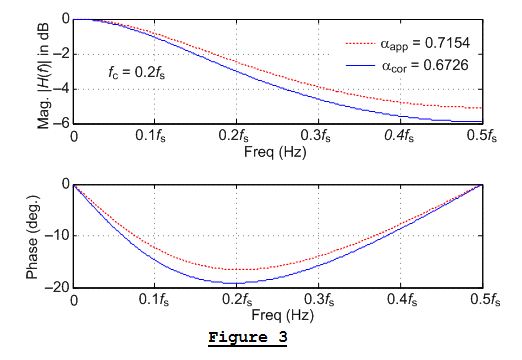
It turns out that the Eq. (1) approximation formula is only reasonably accurate at low values of f_c. As the f_c cutoff frequency is increased in value the greater is the error when using Eq. (1), as shown in Figure 3.

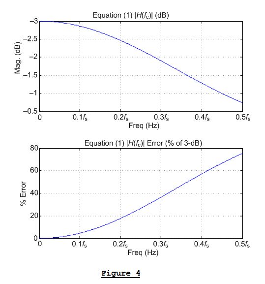
The bottom line of this blog is that the Eq. (1) expression gives reasonably accurate results when the f_c cutoff frequency is less than 0.1f_s. Equation (2) gives exactly correct results regardless of the f_c value.

REFERENCES
[1] V. Vassilevsky, “Efficient Multi-tone Detection,” IEEE Signal
     Processing Magazine, “DSP Tips & Tricks” column, March 2007.
[2] R. Lyons, “Understanding Digital Signal Processing”, 3rd
     Edition, Prentice Hall Publishing, 2011, pp. 789-780.
[3] Pages 613-614 of Reference [2].

APPENDIX A – Deriving Equation (2)
Here's how to derive Eq. (2). The expression for the frequency magnitude response of an exponential averager is [3]:

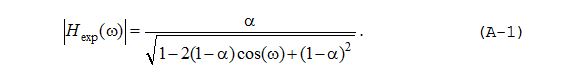
where frequency ω is a normalized angle in the range of 0 ≤ ω ≤ π (corresponding to a continuous-time frequency range of 0 –to- f_s/2 Hz).

So the question is, "What's the expression for α, in terms of ω, so that |H_exp(ω)| = 1/sqrt(2) = 0.707?" If we square Eq. (A-1) and set |H_exp(ω)|² = 0.5, we end up with:

Equation (A-2) can be written as:

Using the quadratic equation we can solve Eq. (A-3) for α as:

where ω = 2Πf_c/f_s, and f_c is the 3-dB cutoff frequency in Hz. Regarding the plus and minus signs before the square root, we choose to use the plus sign for Eq. (2). Choosing the negative sign in Eq. (A-4) places the exponential averager's z-domain pole outside the unit circle. This is a bad thing.

Sign in